Plotting the OGGM surface mass-balance, the ELA and AAR

A few recipes to help you to plot and analyse the mass-balance (MB) computed by OGGM.

import os
import matplotlib.pyplot as plt
import pandas as pd
import xarray as xr
import numpy as np
import pandas as pd

import oggm
from oggm import cfg, utils, workflow, tasks, graphics, global_tasks, DEFAULT_BASE_URL
from oggm.core import massbalance, flowline

cfg.initialize(logging_level='WARNING')
cfg.PATHS['working_dir'] = utils.gettempdir(dirname='OGGM-ref-mb', reset=True)
cfg.PARAMS['border'] = 80
cfg.PARAMS['store_model_geometry'] = True

2024-04-25 13:49:50: oggm.cfg: Reading default parameters from the OGGM `params.cfg` configuration file.
2024-04-25 13:49:50: oggm.cfg: Multiprocessing switched OFF according to the parameter file.
2024-04-25 13:49:50: oggm.cfg: Multiprocessing: using all available processors (N=4)
2024-04-25 13:49:51: oggm.cfg: PARAMS['store_model_geometry'] changed from `False` to `True`.

We use Hintereisferner:

# (The second glacier here we will only use in the second part of this notebook.)
# in OGGM v1.6 you have to explicitly indicate the url from where you want to start from
# we will use here the centerlines to actually look at different flowlines
base_url = ('https://cluster.klima.uni-bremen.de/~oggm/gdirs/oggm_v1.6/'
            'L3-L5_files/2023.1/centerlines/W5E5/')
gdirs = workflow.init_glacier_directories(['RGI60-11.00897', 'RGI60-11.00001'], from_prepro_level=4,
                                          prepro_base_url=DEFAULT_BASE_URL)
# when using centerlines, the new default `SemiImplicit` scheme does not work at the moment,
# we have to use the `FluxBased` scheme instead:
cfg.PARAMS['evolution_model'] = 'FluxBased'

gdir = gdirs[0]
tasks.init_present_time_glacier(gdir)

2024-04-25 13:49:52: oggm.workflow: init_glacier_directories from prepro level 4 on 2 glaciers.
2024-04-25 13:49:52: oggm.workflow: Execute entity tasks [gdir_from_prepro] on 2 glaciers
2024-04-25 13:49:53: oggm.cfg: PARAMS['evolution_model'] changed from `SemiImplicit` to `FluxBased`.

With a static geometry

That’s by far the easiest - that is how we mostly test and develop mass-balance models ourselves.

The very easy way

# Get the calibrated mass-balance model - the default is to use OGGM's "MonthlyTIModel"
mbmod = massbalance.MultipleFlowlineMassBalance(gdir)

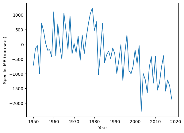
# Compute the specific MB for this glacier
fls = gdir.read_pickle('model_flowlines')
years = np.arange(1950, 2019)
mb_ts = mbmod.get_specific_mb(fls=fls, year=years)

plt.plot(years, mb_ts);
plt.ylabel('Specific MB (mm w.e.)');
plt.xlabel('Year');

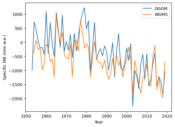
In this particular case (Hintereisferner), we can also plot the measured data:

# Get the reference mass-balance from the WGMS
ref_df = gdir.get_ref_mb_data()
# Get OGGM MB at the same dates
ref_df['OGGM'] = mbmod.get_specific_mb(fls=fls, year=ref_df.index.values)
# Plot
plt.plot(ref_df.index, ref_df.OGGM, label='OGGM');
plt.plot(ref_df.index, ref_df.ANNUAL_BALANCE, label='WGMS');
plt.ylabel('Specific MB (mm w.e.)'); plt.legend();
plt.xlabel('Year');

Mass-balance profiles on flowlines

Let’s start by noting that I used the MultipleFlowlineMassBalance model here. This is what OGGM uses for its runs, because we allow different model parameters for different flowlines. In many cases we don’t need this, but sometimes we do. Let’s see if we have different mass-balance model parameters for Hintereisferner or not. Note, that the new calibration can cause any of the mass-balance model parameters (melt factor, temperature bias or precipitation factor) to be different (more in the massbalance_calibration notebook).

for flmod in mbmod.flowline_mb_models:
    print(flmod.melt_f, f'{flmod.temp_bias:.2f}', f'{flmod.prcp_fac:.2f}')

4.921376081826827 1.76 3.53

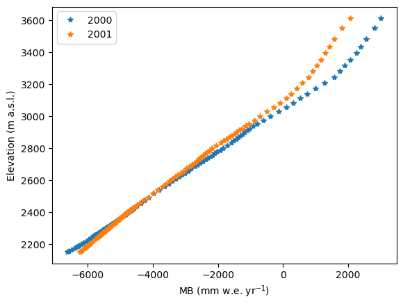
So here we have the same mass-balance model parameters for each flowline (that’s frequently the case). To get the mass-balance as a function of height we have several possibilities:

# Where the flowlines are:
heights, widths, mb = mbmod.get_annual_mb_on_flowlines(fls, year=2000)
# units kg ice per second to mm w.e. per year:
mb = mb * cfg.SEC_IN_YEAR * cfg.PARAMS['ice_density'] 

# Plot
plt.plot(mb, heights, '*', label='2000');

# Another year:
heights, widths, mb = mbmod.get_annual_mb_on_flowlines(fls, year=2001)
# units kg ice per second to mm w.e. per year:
mb = mb * cfg.SEC_IN_YEAR * cfg.PARAMS['ice_density'] 
# Plot
plt.plot(mb, heights, '*', label='2001');
plt.ylabel('Elevation (m a.s.l.)'); plt.xlabel('MB (mm w.e. yr$^{-1}$)'); plt.legend();

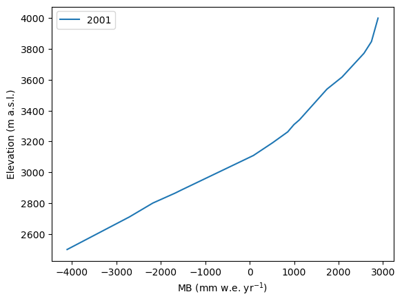
Mass-balance at any height

For this, we can either “pick” one of the single flowline mass-balance models or use the multiple one (it’s the same):

heights = np.arange(2500, 4000)
# Method 1
mbmod1 = mbmod.flowline_mb_models[0]
mb = mbmod1.get_annual_mb(heights, year=2001) * cfg.SEC_IN_YEAR * cfg.PARAMS['ice_density'] 
# Method 2
mb2 = mbmod.get_annual_mb(heights, year=2001, fl_id=0) * cfg.SEC_IN_YEAR * cfg.PARAMS['ice_density'] 
np.testing.assert_allclose(mb, mb2)
# Plot
plt.plot(mb, heights, label='2001');
plt.ylabel('Elevation (m a.s.l.)'); plt.xlabel('MB (mm w.e. yr$^{-1}$)'); plt.legend();

But again, for certain glaciers the mass-balance might change from one flowline to another!

Mass-balance during a transient run + bonus info (timestamps in OGGM)

Specific (glacier-wide) mass-balance

At the time of writing, we only store the glacier volume, which is roughly equivalent to the mass-balance (up to numerical accuracy in the dynamical model).

# We want to use these flowline files for the AAR (see later)
cfg.PARAMS['store_fl_diagnostics'] = True
# Run from outline inventory year (2003 for HEF) to 2017 (end of CRU data in hydro year convention, see below)
tasks.run_from_climate_data(gdir, ye=2020);

2024-04-25 13:49:54: oggm.cfg: PARAMS['store_fl_diagnostics'] changed from `False` to `True`.

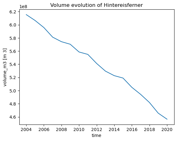
ds_diag = xr.open_dataset(gdir.get_filepath('model_diagnostics'))
ds_diag.volume_m3.plot(); plt.title('Volume evolution of Hintereisferner');

Important: timestamps in OGGM

OGGM was initially developed to follow the traditional “hydrological year” convention. Since OGGM v1.6 or even earlier, we stopped using the hydrological year operationally and use instead simple calendar years. One of the reasons is that our geodetic data used for calibration are also in calendar years. We still give the hydrological year in output files, therefore we introduce it shortly:

We use what we call a “floating year” time stamp, which can be converted to real dates easily in the model:

from oggm.utils import floatyear_to_date, hydrodate_to_calendardate
print('Hydro dates')
print(floatyear_to_date(2003.0))
print(floatyear_to_date(2003.99))
print('Calendar dates')
print(hydrodate_to_calendardate(*floatyear_to_date(2003.0), start_month=10))
print(hydrodate_to_calendardate(*floatyear_to_date(2003.99), start_month=10))

Hydro dates
(2003, 1)
(2003, 12)
Calendar dates
(2002, 10)
(2003, 9)

The timestamp used in the OGGM output files uses the same convention:

# calendar year and month
print(ds_diag.time.values[0], ds_diag.calendar_year.values[0], ds_diag.calendar_month.values[0])

2004.0 2004 1

# hydro year and month
print(ds_diag.time.values[0], ds_diag.hydro_year.values[0], ds_diag.hydro_month.values[0])

2004.0 2004 4

So the simulation started in January 2004 (calendar year: 2004.0), which corresponds to the hydrological year 2004 and month 4, as the hydrological year 2004 starts in October 2003 in the Northern Hemisphere. This is almost in accordance with the RGI inventory date (probably based on satellite imagery taken in the summer 2003):

gdir.rgi_date

2003

Similarly, the simulation ends at the last possible date for which we have climate data for (i.e. the simulation stops at the end of December 2019):

print(ds_diag.time.values[-1], ds_diag.calendar_year.values[-1], ds_diag.calendar_month.values[-1])

2020.0 2020 1

print(ds_diag.time.values[-1], ds_diag.hydro_year.values[-1], ds_diag.hydro_month.values[-1])

2020.0 2020 4

When interpreting the data or reporting them to others, be careful and mention which convention you use. For the moment, it is best to use the simple calendar years.

Specific mass-balance from volume change time series

We compute the specific mass-balance from the delta volume divided by the glacier area, and compare it to observations and to the mass-balance computed with a fixed geometry:

# Specific MB over time (i.e. with changing geometry feedbacks)
smb = (ds_diag.volume_m3.values[1:] - ds_diag.volume_m3.values[:-1]) / ds_diag.area_m2.values[1:]
smb = smb * cfg.PARAMS['ice_density']  # in mm
plt.plot(ds_diag.time[:-1], smb, label='OGGM (dynamics)'); 
# The SMB from WGMS and fixed geometry we already have
plt.plot(ref_df.loc[2004:].index, ref_df.loc[2004:].OGGM, label='OGGM (fixed geom)');
plt.plot(ref_df.loc[2004:].index, ref_df.loc[2004:].ANNUAL_BALANCE, label='WGMS');
plt.legend();

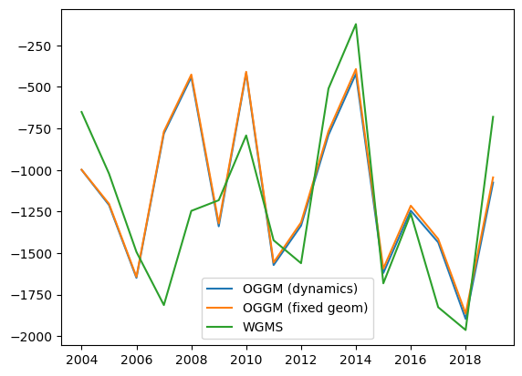
A few comments:

• the systematic difference between WGMS and OGGM is due to the calibration of the model, which is done with fixed geometry (the bias is zero over the entire calibration period but changes sign over the 50 year period, see plot above)

• the difference between OGGM dynamics and fixed geometry (so small that they are barely visible for this short time period) is due to:

  • the changes in geometry during the simulation time (i.e. this difference grows with time)

  • melt at the tongue which might be larger than the glacier thickness is not accounted for in the fixed geometry data (these are assumed to be small)

  • numerical differences in the dynamical model (these are assumed to be small as well)

Mass-balance profiles

At time of writing, we do not store the mass-balance profiles during a transient run, although we could (and should). To get the profiles with a dynamically changing geometry, there is no other way than either get the mass-balance during the simulation, or to fetch the model output and re-compute the mass-balance retroactively.

Note: the mass-balance profiles themselves of course are not really affected by the changing geometry - what changes from one year to another is the altitude at which the model will compute the mass-balance. In other terms, if you are interested in the mass-balance profiles you are better of to use the fixed geometries approaches explained at the beginning of the notebook.

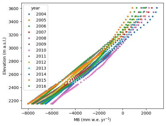
Retrospective mass-balance from model output

# This reads the model output file and makes it look like an OGGM flowline model
dyn_mod = flowline.FileModel(gdir.get_filepath('model_geometry'))
# Get the calibrated mass-balance model
mbmod = massbalance.MultipleFlowlineMassBalance(gdir)
# We can loop over the years and read the flowlines for each year
for year in range(2004, 2017):
    dyn_mod.run_until(year)
    # Compute the SMB from the mass balance model and the flowlines heights at each year
    h = []
    smb = []
    for fl_id, fl in enumerate(dyn_mod.fls):
        h = np.append(h, fl.surface_h)
        mb = mbmod.get_annual_mb(fl.surface_h, year=year, fl_id=fl_id) 
        smb = np.append(smb, mb * cfg.SEC_IN_YEAR * cfg.PARAMS['ice_density'] )
    plt.plot(smb, h, '.', label=year)

plt.legend(title='year');
plt.ylabel('Elevation (m a.s.l.)'); plt.xlabel('MB (mm w.e. yr$^{-1}$)');

Compute the mass-balance during the simulation

# TODO - add the same, but based on the new flowline outputs (like for AAR below)

Equilibrium Line Altitude

The second part of this notebook shows how you can compute the Equilbrium Line Altitude (ELA, the altitude at which the mass-balance is equal to 0) with OGGM.

As the ELA in OGGM only depends on the mass balance model itself (not on glacier geometry), there is no need to do a full model run to collect these values. This is also the reason why the ELA is no longer a part of the model run output, but is instead a diagnostic variable that can be computed separately since OGGM v1.6.

Compute and compile the ELA

global_tasks.compile_ela(gdirs, ys=2000, ye=2019);

2024-04-25 13:49:55: oggm.utils: Applying global task compile_ela on 2 glaciers
2024-04-25 13:49:55: oggm.workflow: Execute entity tasks [compute_ela] on 2 glaciers

Per default, the file will be stored in the working directory and named ELA.hdf (you can choose to save the data in a csv file instead by setting the csv keyword to True). The location where the file is saved can be changed by specifying the path keyword.

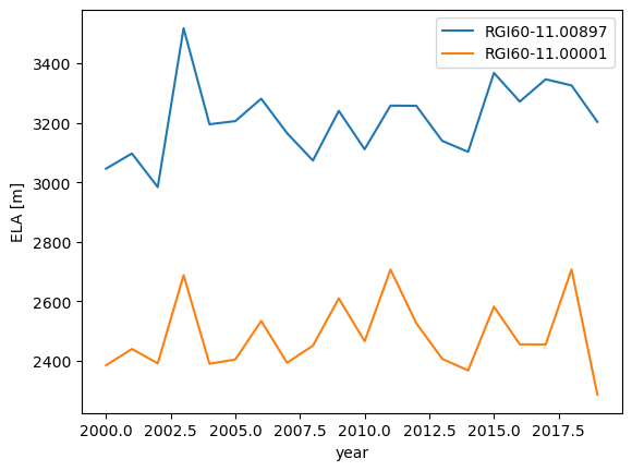
Let’s read the file and plot it:

# Read the file
ela_df = pd.read_hdf(os.path.join(cfg.PATHS['working_dir'], 'ELA.hdf'))

# Plot it
ela_df.plot();
plt.xlabel('year'); plt.ylabel('ELA [m]');

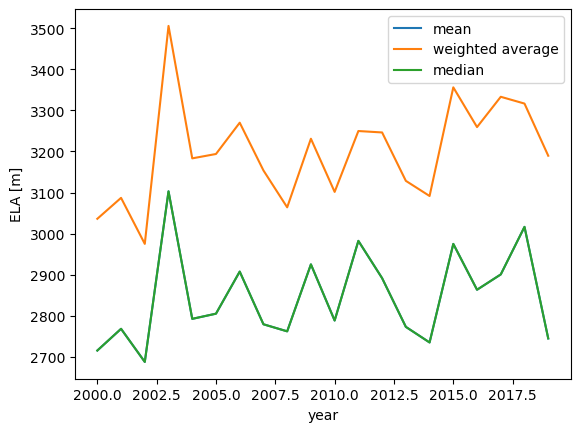
When looking at many glaciers it might be useful to also plot the mean or average of the data. Let’s plot the mean ELA and the glacier area weighted ELA average. Of course, if you only use a few glaciers, as here, it can be much more robust to use the median instead. In the code below, median and mean are the same, because we just used two glaciers ;-) :

areas = [gd.rgi_area_km2 for gd in gdirs]

avg = ela_df.mean(axis=1).to_frame(name='mean')
avg['weighted average'] = np.average(ela_df, axis=1, weights=areas)
avg['median'] = np.median(ela_df, axis=1)

avg.plot();
plt.xlabel('year'); plt.ylabel('ELA [m]');

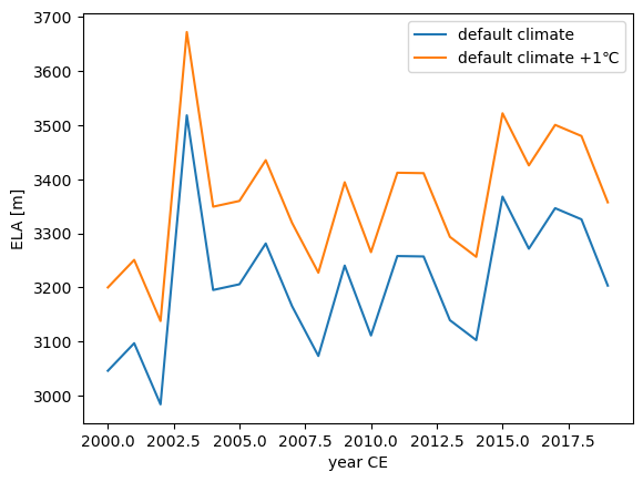
How would the ELA look like if the climate is 1° warmer? Lets have a look at one of the glaciers:

mbmod = massbalance.MonthlyTIModel(gdir, filename='climate_historical')

mbmod

<oggm.MassBalanceModel>
  Class: MonthlyTIModel
  Attributes:
    - hemisphere: nh
    - climate_source: GSWP3_W5E5
    - melt_f: 4.92
    - prcp_fac: 3.53
    - temp_bias: 1.76
    - bias: 0.00
    - rho: 900.0
    - t_solid: 0.0
    - t_liq: 2.0
    - t_melt: -1.0
    - repeat: False
    - ref_hgt: 2252.0
    - ys: 1901
    - ye: 2019

# We first need to get the currently applied temperature bias (that corrects for biases
# in the local climate) and then we add the additional temperature bias on top of it 
# (note that since OGGM v1.6, the calibrated temp_bias is very likely to be 
# different for every glacier)
corr_temp_bias = gdirs[0].read_json('mb_calib')['temp_bias']
corr_temp_bias

1.7583130779353044

global_tasks.compile_ela(gdirs[0], ys=2000, ye=2019,
                        temperature_bias=corr_temp_bias+1,
                        filesuffix='_t1')
ela_df_t1 = pd.read_hdf(os.path.join(cfg.PATHS['working_dir'], 'ELA_t1.hdf'))

2024-04-25 13:49:56: oggm.utils: Applying global task compile_ela on 1 glaciers
2024-04-25 13:49:56: oggm.workflow: Execute entity tasks [compute_ela] on 1 glaciers

# we only look at the first glacier
plt.plot(ela_df[[ela_df.columns[0]]].mean(axis=1), label='default climate')
plt.plot(ela_df_t1.mean(axis=1), label=('default climate +1℃'))
plt.xlabel('year CE'); plt.ylabel('ELA [m]'); plt.legend();

By using the precipitation_factor keyword, you can change the precipitation. Feel free to try that by yourself! At the moment, gdirs[0].read_json('mb_calib')['prcp_fac'] is applied.

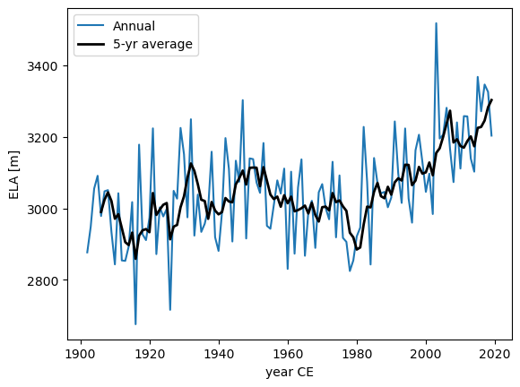
Lets look at a longer timeseries, for one glacier only:

global_tasks.compile_ela(gdirs[0], ys=1902, ye=2019, filesuffix='_1901_2019', csv=True)
ela_df_long = pd.read_csv(os.path.join(cfg.PATHS['working_dir'], 'ELA_1901_2019.csv'),
                          index_col=0)

2024-04-25 13:49:56: oggm.utils: Applying global task compile_ela on 1 glaciers
2024-04-25 13:49:56: oggm.workflow: Execute entity tasks [compute_ela] on 1 glaciers

The ELA can have a high year-to-year variability. Therefore we plot in addition to the regular ELA timeseries, the 5-year moving average.

ax = ela_df_long.plot();
ela_df_long.rolling(5).mean().plot(ax=ax, lw=2, color='k', label='')
plt.xlabel('year CE'); plt.ylabel('ELA [m]'); ax.legend(["Annual", "5-yr average"]);

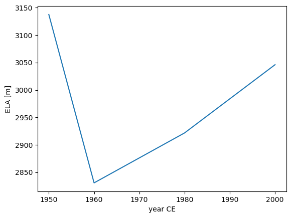
In case you’re only intrested in specific years there is an option to just compute the ELA in those years. There is actually no need to save this data. Therefore we now just compute the ELA.

yrs = [2000, 1950, 1980, 1960]
ela_yrs = massbalance.compute_ela(gdirs[0], years=yrs)
ela_yrs

2000    3046.143863
1950    3137.663937
1980    2921.696602
1960    2830.612223
dtype: float64

See in this case you can use any year as long as you have climate available for that year. However for plotting purposes it might be worth to sort the data, otherwise the following happens ;)

ela_yrs.plot();

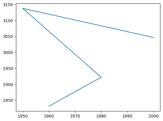
ela_yrs.sort_index(ascending=True).plot();
plt.xlabel('year CE'); plt.ylabel('ELA [m]');

By now we have addressed most of the keyword agruments of the compile_ela and compute_ela functions. To use different climate than the default climate, you can make use of the climate_filename and climate_input_filesuffix keywords. In case you’re not familiar with those yet, please check out the run_with_gcm notebook.

Accumulation Area Ratio

Like the ELA, the Accumulation Area Ratio (AAR) is a diagostic variable. The AAR is currently not an output variable in OGGM, but it can easily be computed. It is even a part of the glacier simulator and its documentation. Below we give an example of how it can be computed after a model run. From the ELA computation, we already know the height where the mass balance is equal to zero. Now we need to compute the area of the glacier that is located above that line. Let’s start with a static geometry glacier with multiple flowlines.

We first search the points along the flowlines that are above the ELA in a given year. Lets use Hintereisferner.

We use a True, False array saying which part is above the ELA and sum the corresponding area at each timestep:

rgi_id = 'RGI60-11.00897'

tot_area = 0
tot_area_above = 0
for fl in fls:
    # The area is constant
    tot_area += fl.area_m2
    # The area above a certain limit is not - we make a (nx, nt) array
    # This is a little bit of dimensional juggling (broadcasting)
    is_above = (fl.surface_h[:, np.newaxis, ] > ela_df[rgi_id].values)
    # Here too - but the time dim is constant
    area = fl.bin_area_m2[:, np.newaxis] * np.ones(len(ela_df))
    tot_area_above += (area * is_above).sum(axis=0)

# Write the output
fixed_aar = pd.DataFrame(index=ela_df.index)
fixed_aar['AAR'] = tot_area_above / tot_area

# Plot ELA and AAR on the same plot
fixed_aar['ELA'] = ela_df[rgi_id]
fixed_aar.plot(secondary_y='ELA');

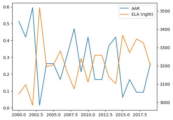
Unsurprisingly, the AAR is strongly correlated to the ELA, but it is not fully linear due to the area distribution of the glacier:

fixed_aar.plot.scatter(x='AAR', y='ELA');

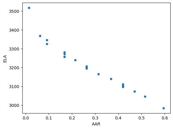
Now that we have looked at the static case, let’s to the same for glaciers with changing surface height:

# We start by reading the flowline geometry diagnostic files
tot_area = 0
tot_area_above = 0

ela_ds = xr.DataArray(ela_df[rgi_id], dims=('time'))

for fn in np.arange(len(fls)):
    with xr.open_dataset(gdir.get_filepath('fl_diagnostics'), group='fl_' + str(fn)) as ds:
        ds = ds.load()
    tot_area += ds.area_m2.sum(dim='dis_along_flowline')

    # Compute the surface elevation
    surface_h = ds.thickness_m + ds.bed_h

    # In xarray things are much easier - the broadcasting is automatic
    is_above = surface_h > ela_ds
    area = is_above * ds.area_m2
    tot_area_above += (area * is_above).sum(dim='dis_along_flowline')

# Write the output
dyna_aar = pd.DataFrame(index=tot_area_above.time)
dyna_aar['AAR_dyna'] = tot_area_above / tot_area
dyna_aar['AAR_fixed'] = fixed_aar['AAR']

dyna_aar.plot(); plt.ylabel('AAR');

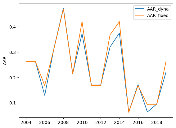
You can see in the plot that the difference between the AAR calculated from the dynamic glacier and the one of the static glacier is quite similar. Over time you can expect that this difference becomes larger. Feel free to play around with that.

Keep in mind that this is just an example for computing the AAR. For a different glacier experiment you might need to adjust the code. e.g. if the glacier flowlines would have different MB model parameters, you need to take that in to consideration.

Here we computed the AAR from the “model perspective”, where the glacier is located in bins. You can however also choose to do some interpolation between the grid point above and below the ELA.

What’s next?

• look at the OGGM-Shop documentation

• back to the table of contents