Differences between the “elevation band” and “centerline” flowlines#
In version 1.4, OGGM introduced a new way to compute flowlines: the so-called “elevation-band flowlines” (after Huss & Farinotti, 2012). These elevation bands complement the already available “multiple centerlines” glacier representation.
In OGGM 1.6 and above, the “elevation band” representation is the most commonly used representation for large scale simulations.
This notebook allows you to compare the two representations. It shows that the difference between the two are small for projections of glacier change, but each representation comes with pros and cons when it comes to single glacier simulations.
Tags: beginner, workflow, dynamics, flowlines
from oggm import cfg, utils, workflow, graphics, tasks
import xarray as xr
import numpy as np
import matplotlib.pyplot as plt
import seaborn as sns
cfg.initialize(logging_level='WARNING')
2024-04-25 13:19:42: oggm.cfg: Reading default parameters from the OGGM `params.cfg` configuration file.
2024-04-25 13:19:42: oggm.cfg: Multiprocessing switched OFF according to the parameter file.
2024-04-25 13:19:42: oggm.cfg: Multiprocessing: using all available processors (N=4)
# Pick the glacier you want! We use Baltoro here
rgi_ids = ['RGI60-14.06794']
Get ready#
In order to open the same glacier on two different glacier directories, we apply a trick: we set a new working directory for each case! This trick is not recommended for real runs: if you have a use case for such a workflow (the same glacier with different flowline types, please get in touch with us).
# Geometrical centerline
# Where to store the data
cfg.PATHS['working_dir'] = utils.gettempdir(dirname='OGGM-centerlines', reset=True)

# We start from prepro level 3 with all data ready - note the url here
base_url = 'https://cluster.klima.uni-bremen.de/~oggm/gdirs/oggm_v1.6/L3-L5_files/2023.3/centerlines/W5E5/'
gdirs = workflow.init_glacier_directories(rgi_ids, from_prepro_level=3, prepro_border=80, prepro_base_url=base_url)
gdir_cl = gdirs[0]
gdir_cl
2024-04-25 13:19:43: oggm.workflow: init_glacier_directories from prepro level 3 on 1 glaciers.
2024-04-25 13:19:43: oggm.workflow: Execute entity tasks [gdir_from_prepro] on 1 glaciers
<oggm.GlacierDirectory>
  RGI id: RGI60-14.06794
  Region: 14: South Asia West
  Subregion: 14-02: Karakoram
  Name: Baltoro Glacier
  Glacier type: Glacier
  Terminus type: Land-terminating
  Status: Glacier or ice cap
  Area: 809.109 km2
  Lon, Lat: (76.4047, 35.7416)
  Grid (nx, ny): (479, 346)
  Grid (dx, dy): (200.0, -200.0)
# Elevation band flowline
# New working directory
cfg.PATHS['working_dir'] = utils.gettempdir(dirname='OGGM-elevbands', reset=True)

# Note the new url
base_url = 'https://cluster.klima.uni-bremen.de/~oggm/gdirs/oggm_v1.6/L3-L5_files/2023.3/elev_bands/W5E5/'
gdirs = workflow.init_glacier_directories(rgi_ids, from_prepro_level=3, prepro_border=80, prepro_base_url=base_url)
gdir_eb = gdirs[0]
gdir_eb
2024-04-25 13:19:59: oggm.workflow: init_glacier_directories from prepro level 3 on 1 glaciers.
2024-04-25 13:19:59: oggm.workflow: Execute entity tasks [gdir_from_prepro] on 1 glaciers
<oggm.GlacierDirectory>
  RGI id: RGI60-14.06794
  Region: 14: South Asia West
  Subregion: 14-02: Karakoram
  Name: Baltoro Glacier
  Glacier type: Glacier
  Terminus type: Land-terminating
  Status: Glacier or ice cap
  Area: 809.109 km2
  Lon, Lat: (76.4047, 35.7416)
  Grid (nx, ny): (479, 346)
  Grid (dx, dy): (200.0, -200.0)
Some reading first#
We wrote a bit of information about the differences between these two. First, go to the glacier flowlines documentation where you can find detailed information about the two flowline types and also a guideline when to use which flowline method.
The examples below illustrate these differences, without much text for now because of lack of time:
Glacier length and cross section#
fls_cl = gdir_cl.read_pickle('model_flowlines')
fls_eb = gdir_eb.read_pickle('model_flowlines')
f, (ax1, ax2) = plt.subplots(2, 1, figsize=(10, 14), sharex=True, sharey=True)
graphics.plot_modeloutput_section(fls_cl, ax=ax1)
ax1.set_title('Geometrical centerline')
graphics.plot_modeloutput_section(fls_eb, ax=ax2)
ax2.set_title('Elevation band flowline');
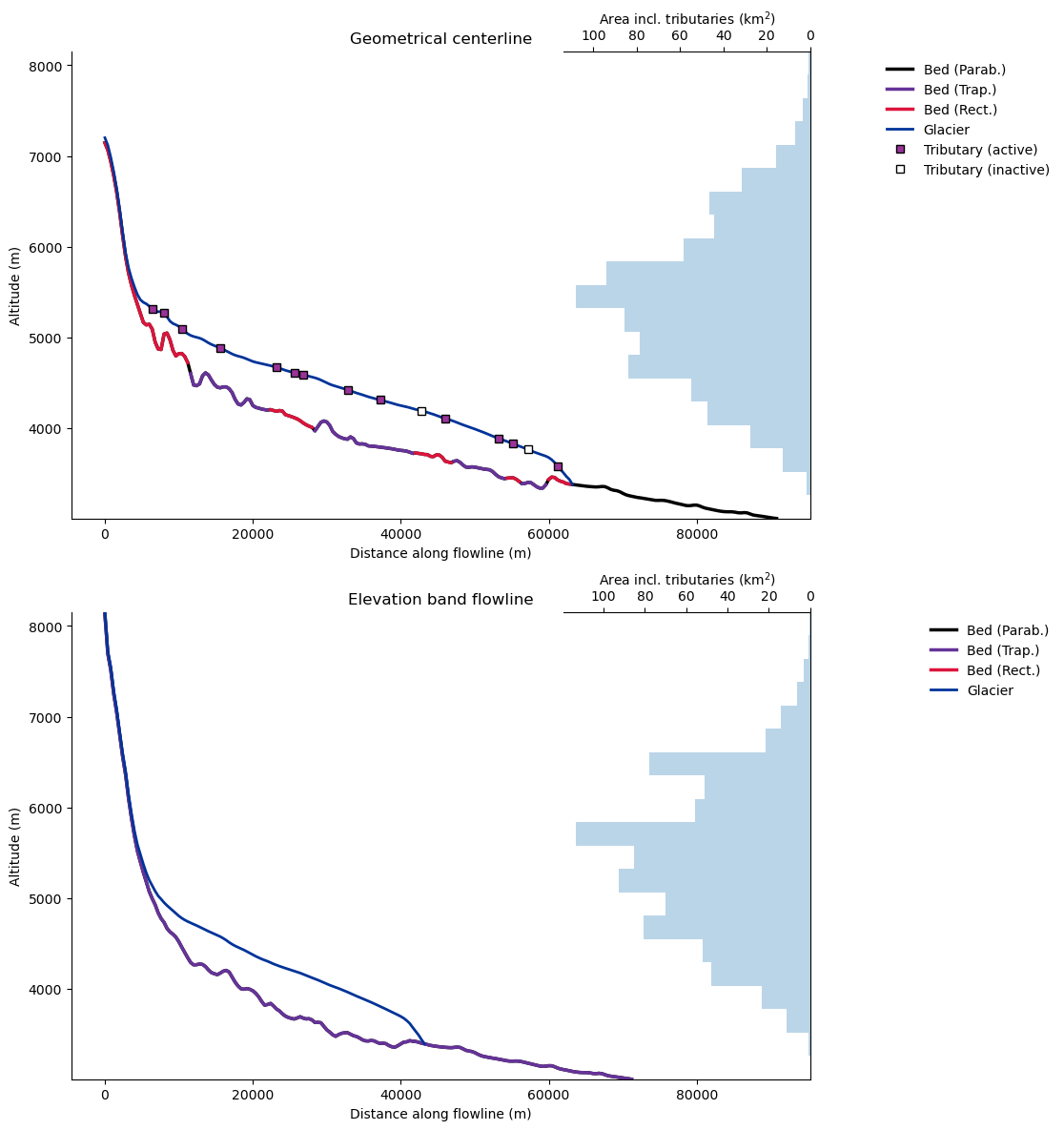
Note that the elevation band flowline length is shorter than the geometrical centerline!
Projections: generally small differences in volume, but larger differences in geometry (length and area)#
Thanks to OGGM’s modular workflow, a simulation with each geometry is fairly similar in terms of code. For example, we can process the climate data for both representations with the same command:
gdirs = [gdir_cl, gdir_eb]
from oggm.shop import gcm_climate

# you can choose one of these 5 different GCMs:
# 'gfdl-esm4_r1i1p1f1', 'mpi-esm1-2-hr_r1i1p1f1', 'mri-esm2-0_r1i1p1f1' ("low sensitivity" models, within typical ranges from AR6)
# 'ipsl-cm6a-lr_r1i1p1f1', 'ukesm1-0-ll_r1i1p1f2' ("hotter" models, especially ukesm1-0-ll)
member = 'mri-esm2-0_r1i1p1f1'

for ssp in ['ssp126', 'ssp370','ssp585']:
    # bias correct them
    workflow.execute_entity_task(gcm_climate.process_monthly_isimip_data, gdirs,
                                 ssp = ssp,
                                 # gcm member -> you can choose another one
                                 member=member,
                                 # recognize the climate file for later
                                 output_filesuffix=f'_ISIMIP3b_{member}_{ssp}'
                                 );
2024-04-25 13:20:14: oggm.workflow: Execute entity tasks [process_monthly_isimip_data] on 2 glaciers
2024-04-25 13:20:16: oggm.workflow: Execute entity tasks [process_monthly_isimip_data] on 2 glaciers
2024-04-25 13:20:18: oggm.workflow: Execute entity tasks [process_monthly_isimip_data] on 2 glaciers
For the ice dynamics simulations, the commands are exactly the same as well. The only difference is that centerlines require the more flexible “FluxBased” numerical model, while the elevation bands can also use the more robust “SemiImplicit” one. The runs are considerabily faster with the elevation bands flowlines.
# add additional outputs to default OGGM
cfg.PARAMS['store_model_geometry'] = True
cfg.PARAMS['store_fl_diagnostics'] = True

for gdir in gdirs:
    if gdir is gdir_cl:
        cfg.PARAMS['evolution_model'] = 'FluxBased'
    else:
        cfg.PARAMS['evolution_model'] = 'SemiImplicit'

    workflow.execute_entity_task(tasks.run_from_climate_data, [gdir],
                                 output_filesuffix='_historical',
                                );

    for ssp in ['ssp126', 'ssp370', 'ssp585']:
        rid = f'_ISIMIP3b_{member}_{ssp}'

        workflow.execute_entity_task(tasks.run_from_climate_data, [gdir],
                                     climate_filename='gcm_data',  # use gcm_data, not climate_historical
                                     climate_input_filesuffix=rid,  # use the chosen scenario
                                     init_model_filesuffix='_historical',  # this is important! Start from 2020 glacier
                                     output_filesuffix=rid,  # recognize the run for later
                                    );
2024-04-25 13:20:19: oggm.cfg: PARAMS['store_model_geometry'] changed from `False` to `True`.
2024-04-25 13:20:19: oggm.cfg: PARAMS['store_fl_diagnostics'] changed from `False` to `True`.
2024-04-25 13:20:19: oggm.cfg: PARAMS['evolution_model'] changed from `SemiImplicit` to `FluxBased`.
2024-04-25 13:20:19: oggm.workflow: Execute entity tasks [run_from_climate_data] on 1 glaciers
2024-04-25 13:20:36: oggm.workflow: Execute entity tasks [run_from_climate_data] on 1 glaciers
2024-04-25 13:21:24: oggm.workflow: Execute entity tasks [run_from_climate_data] on 1 glaciers
2024-04-25 13:22:10: oggm.workflow: Execute entity tasks [run_from_climate_data] on 1 glaciers
2024-04-25 13:22:56: oggm.cfg: PARAMS['evolution_model'] changed from `FluxBased` to `SemiImplicit`.
2024-04-25 13:22:56: oggm.workflow: Execute entity tasks [run_from_climate_data] on 1 glaciers
2024-04-25 13:22:56: oggm.workflow: Execute entity tasks [run_from_climate_data] on 1 glaciers
2024-04-25 13:22:56: oggm.workflow: Execute entity tasks [run_from_climate_data] on 1 glaciers
2024-04-25 13:22:57: oggm.workflow: Execute entity tasks [run_from_climate_data] on 1 glaciers
f, (ax1, ax2) = plt.subplots(1, 2, figsize=(14, 4))

# Pick some colors for the lines
color_dict={'ssp126':'blue', 'ssp370':'orange', 'ssp585':'red'}

for ssp in ['ssp126','ssp370', 'ssp585']:
    rid = f'_ISIMIP3b_{member}_{ssp}'
    with xr.open_dataset(gdir_cl.get_filepath('model_diagnostics', filesuffix=rid)) as ds:
        ds.volume_m3.plot(ax=ax1, label=ssp, c=color_dict[ssp]);
for ssp in ['ssp126','ssp370', 'ssp585']:
    rid = f'_ISIMIP3b_{member}_{ssp}'
    with xr.open_dataset(gdir_eb.get_filepath('model_diagnostics', filesuffix=rid)) as ds:
        ds.volume_m3.plot(ax=ax1, label=ssp, c=color_dict[ssp], ls='--');
    ax1.set_title('Glacier volume')
    ax1.set_xlim([2020,2100])
    ax1.set_ylim([0, ds.volume_m3.max().max()*1.1])

for ssp in ['ssp126','ssp370', 'ssp585']:
    rid = f'_ISIMIP3b_{member}_{ssp}'
    with xr.open_dataset(gdir_cl.get_filepath('model_diagnostics', filesuffix=rid)) as ds:
        ds.length_m.plot(ax=ax2, label=ssp, c=color_dict[ssp]);
    ax2.set_ylim([0, ds.length_m.max().max()*1.1])
for ssp in ['ssp126','ssp370', 'ssp585']:
    rid = f'_ISIMIP3b_{member}_{ssp}'
    with xr.open_dataset(gdir_eb.get_filepath('model_diagnostics', filesuffix=rid)) as ds:
        ds.length_m.plot(ax=ax2, label=ssp, c=color_dict[ssp], ls='--');
    ax2.set_title('Glacier length')
    ax2.set_xlim([2020,2100])

plt.legend();
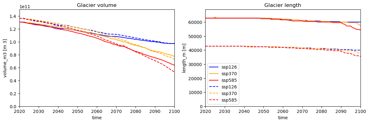
As you can see, for this disappearing glacier, the representations create slightly different volume projections. The differences can be quite a bit larger at times, for example for length projections.
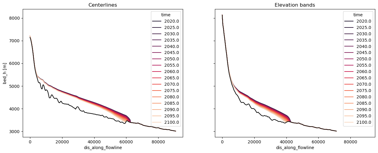
Graphical representation: centerlines win by short margin (for now)#
rid = f'_ISIMIP3b_{member}_ssp126'
Both models can be reprensented with a cross-section, like this:
sel_years = np.linspace(2020, 2100, 17).astype(int)
colors = sns.color_palette('rocket', len(sel_years))
with plt.rc_context({'axes.prop_cycle': plt.cycler(color=colors)}):
    f, (ax1, ax2) = plt.subplots(1, 2, figsize=(15, 5.5), sharey=True, sharex=True)
    n_lines = len(gdir_cl.read_pickle('model_flowlines'))
    with xr.open_dataset(gdir_cl.get_filepath('fl_diagnostics', filesuffix=rid), group=f'fl_{n_lines-1}') as ds:
        (ds.bed_h + ds.sel(time=sel_years).thickness_m).plot(ax=ax1, hue='time')
        ds.bed_h.plot(ax=ax1, c='k')
        ax1.set_title('Centerlines')
    with xr.open_dataset(gdir_eb.get_filepath('fl_diagnostics', filesuffix=rid), group='fl_0') as ds:
        (ds.bed_h + ds.sel(time=sel_years).thickness_m).plot(ax=ax2, hue='time')
        ds.bed_h.plot(ax=ax2, c='k')
        ax2.set_ylabel('')
        ax2.set_title('Elevation bands')
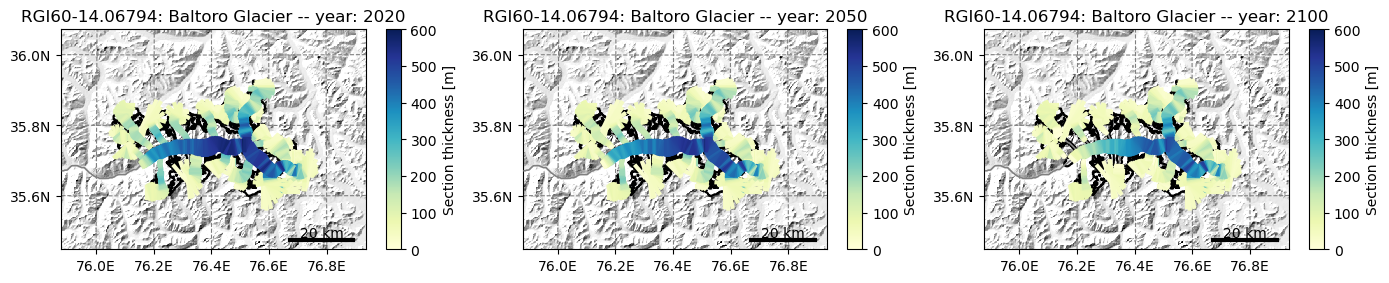
However, only centerlines can be plotted as a map:
# this can take some time
# if you want to see more thickness differences you can use ssp585 instead of ssp126
# by uncomment the following line
# rid = f'_ISIMIP3b_{member}_ssp585'
f, (ax1, ax2, ax3) = plt.subplots(1, 3, figsize=(14, 6))
# let's have the same colorbar for every subplot for better comparability
graphics.plot_modeloutput_map(gdir_cl, filesuffix=rid, modelyr=2020, ax=ax1, vmax=600)
graphics.plot_modeloutput_map(gdir_cl, filesuffix=rid, modelyr=2050, ax=ax2, vmax=600)
graphics.plot_modeloutput_map(gdir_cl, filesuffix=rid, modelyr=2100, ax=ax3, vmax=600)
plt.tight_layout();
We are however working on a better representation of retreating glaciers for outreach. Have a look at this tutorial!
Take home messages#
in the absence of additional data to better calibrate the mass balance model, using multiple centerlines is considered not useful: indeed, the distributed representation offers little advantages if the mass balance is only a function of elevation.
elevation band flowlines are now the default of most OGGM applications. It is faster, much cheaper, and more robust to use these simplified glaciers.
elevation band flowlines cannot be represented on a map “out of the box”. We have however developped a tool to display the changes by redistributing them on a map: have a look at this tutorial!
multiple centerlines can be useful for growing glacier cases and use cases where geometry plays an important role (e.g. lakes, paleo applications).
What’s next?#
return to the OGGM documentation
back to the table of contents