Global distribution of the mass-balance model parameters#
This notebook is a follow-up on the very important overview of the mass-balance calibration procedure in v1.6.
Here we illustrate a few useful methods:
checking some statistics on the pre-processed directories (similar to preprocessing_errors.ipynb)
we check how the new global calibration procedure operates
we assess the importance of the dynamical spinup for the calibration
from oggm import utils
import pandas as pd
import numpy as np
import matplotlib.pyplot as plt
import seaborn as sns
Let’s start by reading in the “glacier statistics” files, a bunch of statistics written by OGGM at the end of the preprocessing:
# W5E5 elevbands, no spinup
url = 'https://cluster.klima.uni-bremen.de/~oggm/gdirs/oggm_v1.6/L3-L5_files/2023.3/elev_bands/W5E5/RGI62/b_080/L5/summary/'

# this can take some time to downloan
df = []
for rgi_reg in range(1, 19):
    fpath = utils.file_downloader(url + f'glacier_statistics_{rgi_reg:02d}.csv')
    df.append(pd.read_csv(fpath, index_col=0, low_memory=False))
df = pd.concat(df, sort=False).sort_index()

# There are a lot of columns - let's pick a few columns only
# We drop failing glaciers
df_params = df[['melt_f', 'prcp_fac', 'temp_bias', 'rgi_area_km2']].dropna().copy()
f'Failing glaciers: {len(df) - len(df_params)} ({100 - df_params.rgi_area_km2.sum()/df.rgi_area_km2.sum()*100:.2f}% of global area)'
'Failing glaciers: 718 (0.06% of global area)'
Global statistics of OGGM’s 1.6.1 “informed three steps” method#
As explained in the mass-balance calibration procedure in v1.6 notebook, the “informed three steps” method provides first guesses for the precipitation factor and the temperature bias. We then calibrate each glacier in three steps - let’s check the number of glaciers calibrated this way:
Step 0: use the first guess melt_f = 5, prcp_fac = data-informed from winter precipitation, temp_bias = data-informed from the global calibration with fixed parameters (see mass-balance calibration procedure in v1.6 for details).
Step 1: if Step 0 doesn’t match (only likely to happen if there is one isolated glacier in a climate grid point), allow prcp_fac to vary again between 0.8 and 1.2 times the roiginal guess (\(\pm\)20%). This is justified by the fact that the first guess for precipitation is also highly uncertain. If that worked, the calibration stops.
To find out which glaciers have been calibrated after step 1, we count the number of glaciers with a melt factor of exactly 5:
df_params['Step 1'] = np.isclose(df_params['melt_f'], 5)
perc1 = df_params['Step 1'].sum() / len(df_params) * 100
perc1_area = df_params.loc[df_params['Step 1']].rgi_area_km2.sum()/df.rgi_area_km2.sum()*100
print(f'{perc1:.1f}% of all glaciers are calibrated after step 1 ({perc1_area:.1f}% area)')
33.6% of all glaciers are calibrated after step 1 (41.1% area)
Step 2: if Step 1 did not work, we allow melt_f to vary between a predefined range (1.5 - 17) while fixing temp_bias and prcp_fac again.
Step 3: finally, if the above did not work, allow temp_bias to vary again, fixing the other parameters to their last value.
To check wether these steps were successful from our files, we can compute the number of glaciers which have hit the “hard limits” of the allowed melt factor range, i.e. have reached step 3, and then substract them from the total:
df_params['Step 3'] = np.isclose(df_params['melt_f'], df_params['melt_f'].max()) | np.isclose(df_params['melt_f'], df_params['melt_f'].min())
perc3 = df_params['Step 3'].sum() / len(df_params) * 100
perc3_area = df_params.loc[df_params['Step 3']].rgi_area_km2.sum()/df.rgi_area_km2.sum()*100

df_params['Step 2'] = (~ df_params['Step 1']) & (~ df_params['Step 3'])
perc2 = df_params['Step 2'].sum() / len(df_params) * 100
perc2_area = df_params.loc[df_params['Step 2']].rgi_area_km2.sum()/df.rgi_area_km2.sum()*100

print(f'{perc2:.1f}% of all glaciers are calibrated after step 2 ({perc2_area:.1f}% area)')
print(f'{perc3:.1f}% of all glaciers are calibrated after step 3 ({perc3_area:.1f}% area)')
60.4% of all glaciers are calibrated after step 2 (56.7% area)
5.9% of all glaciers are calibrated after step 3 (2.2% area)
Global parameter distributions#
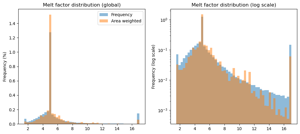
Melt factor#
f, (ax1, ax2) = plt.subplots(1, 2, figsize=(12, 5))

df_params['melt_f'].plot.hist(bins=51, density=True, ax=ax1, alpha=0.5, label='Frequency');
df_params['melt_f'].plot.hist(bins=51, density=True, ax=ax1, weights=df_params['rgi_area_km2'], alpha=0.5, label='Area weighted');
ax1.set_title('Melt factor distribution (global)');
ax1.set_ylabel('Frequency (%)');
ax1.legend();

df_params['melt_f'].plot.hist(bins=51, density=True, ax=ax2, alpha=0.5, label='Frequency');
df_params['melt_f'].plot.hist(bins=51, density=True, ax=ax2, weights=df_params['rgi_area_km2'], alpha=0.5, label='Area weighted');
ax2.set_yscale('log')
ax2.set_title('Melt factor distribution (log scale)');
ax2.set_ylabel('Frequency (log scale)');
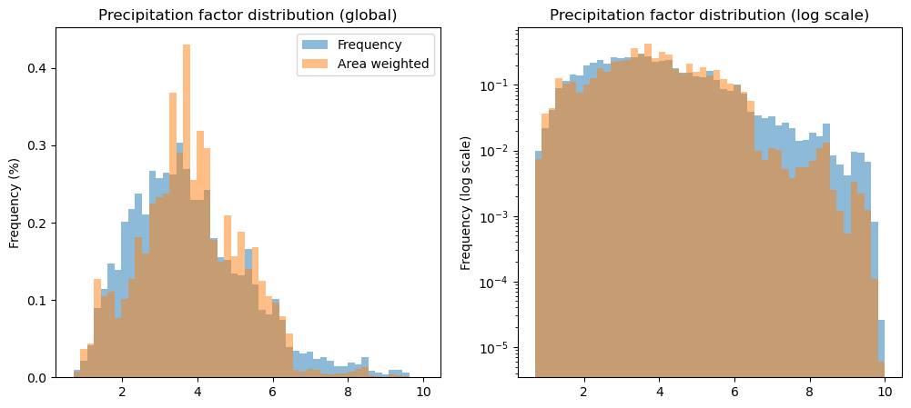
Precip factor#
f, (ax1, ax2) = plt.subplots(1, 2, figsize=(12, 5))

df_params['prcp_fac'].plot.hist(bins=51, density=True, ax=ax1, alpha=0.5, label='Frequency');
df_params['prcp_fac'].plot.hist(bins=51, density=True, ax=ax1, weights=df_params['rgi_area_km2'], alpha=0.5, label='Area weighted');
ax1.set_title('Precipitation factor distribution (global)');
ax1.set_ylabel('Frequency (%)');
ax1.legend();

df_params['prcp_fac'].plot.hist(bins=51, density=True, ax=ax2, alpha=0.5, label='Frequency');
df_params['prcp_fac'].plot.hist(bins=51, density=True, ax=ax2, weights=df_params['rgi_area_km2'], alpha=0.5, label='Area weighted');
ax2.set_yscale('log')
ax2.set_title('Precipitation factor distribution (log scale)');
ax2.set_ylabel('Frequency (log scale)');
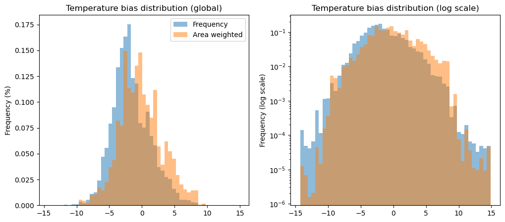
Temperature bias#
f, (ax1, ax2) = plt.subplots(1, 2, figsize=(12, 5))

df_params['temp_bias'].plot.hist(bins=51, density=True, ax=ax1, alpha=0.5, label='Frequency');
df_params['temp_bias'].plot.hist(bins=51, density=True, ax=ax1, weights=df_params['rgi_area_km2'], alpha=0.5, label='Area weighted');
ax1.set_title('Temperature bias distribution (global)');
ax1.set_ylabel('Frequency (%)');
ax1.legend();

df_params['temp_bias'].plot.hist(bins=51, density=True, ax=ax2, alpha=0.5, label='Frequency');
df_params['temp_bias'].plot.hist(bins=51, density=True, ax=ax2, weights=df_params['rgi_area_km2'], alpha=0.5, label='Area weighted');
ax2.set_yscale('log')
ax2.set_title('Temperature bias distribution (log scale)');
ax2.set_ylabel('Frequency (log scale)');
Take home#
a substantial (33%) part of all glaciers are attributed the default melt factor of 5 after the first guesses in climate data bias correction. In other words, this means that we are substantially correcting the climate forcing to “match” the presence of a glacier. Other calibration methods are using similar techniques (they differ in the details and the allowed range of parameter values)
the large amount of glaciers with melt factor of exactly 5 is problematic, but is mitigated somewhat by the dynamical spinup (see below)
the largest bulk of the glacier area is calibrated with “pre-informed” precip factor and temperature bias, and have a calibrated melt factor. The resulting melt factor distribution is centered around 5 and has a long tail towards higher values.
in general, weighting the distributions by area tends to reduce the extremes.
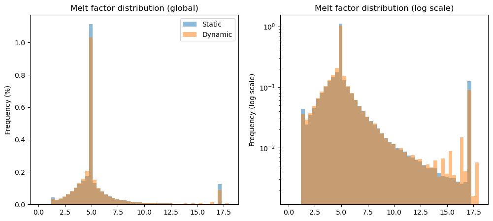
Influence of dynamical spinup#
The dynamical spinup procedure (explained in this 10 minutes tutorial and in more detail in this tutorial) starts from the parameters calibrated above with a static geometry and calibrate the melt factor again using an iterative procedure, making sure that the parameters and the past evolution of the glacier are consistent with the past evolution of the glacier. In doing so, it achieves two things:
the actually modelled mass balance of glaciers during a dynamical run matches observations better than without
it reshuffles the melt factors a bit
Let’s test this second hypothesis by downloading the statistics for the spinup directories:
# W5E5 elevbands, with spinup
url = 'https://cluster.klima.uni-bremen.de/~oggm/gdirs/oggm_v1.6/L3-L5_files/2023.3/elev_bands/W5E5_spinup/RGI62/b_160/L5/summary/'

# this can take some time
dfs = []
for rgi_reg in range(1, 19):
    fpath = utils.file_downloader(url + f'glacier_statistics_{rgi_reg:02d}.csv')
    dfs.append(pd.read_csv(fpath, index_col=0, low_memory=False))
dfs = pd.concat(dfs, sort=False).sort_index()
df_params['melt_f_dyna'] = dfs['melt_f']
First of all, let’s see how many glaciers have had their melt factor changed as a result of the dynamical calibration (i.e. dynamical calibration was succesful):
df_params['dyna_changed'] = ~ np.isclose(df_params['melt_f'], df_params['melt_f_dyna'])
perc = df_params['dyna_changed'].sum() / len(df_params) * 100
perc_area = df_params.loc[df_params['dyna_changed']].rgi_area_km2.sum()/df.rgi_area_km2.sum()*100
print(f'{perc:.1f}% of all glaciers are re calibrated after dynamical spinup ({perc_area:.1f}% area)')
70.3% of all glaciers are re calibrated after dynamical spinup (76.4% area)
Let’s plot the change in distribution of the parameters:
f, (ax1, ax2) = plt.subplots(1, 2, figsize=(12, 5))
bins = np.linspace(0.1, 18, 51)
df_params['melt_f'].plot.hist(bins=bins, density=True, ax=ax1, alpha=0.5, label='Static');
df_params['melt_f_dyna'].plot.hist(bins=bins, density=True, ax=ax1, alpha=0.5, label='Dynamic');
ax1.set_title('Melt factor distribution (global)');
ax1.set_ylabel('Frequency (%)');
ax1.legend();

df_params['melt_f'].plot.hist(bins=bins, density=True, ax=ax2, alpha=0.5, label='Static');
df_params['melt_f_dyna'].plot.hist(bins=bins, density=True, ax=ax2, alpha=0.5, label='Dynamic');
ax2.set_yscale('log')
ax2.set_title('Melt factor distribution (log scale)');
ax2.set_ylabel('Frequency (log scale)');
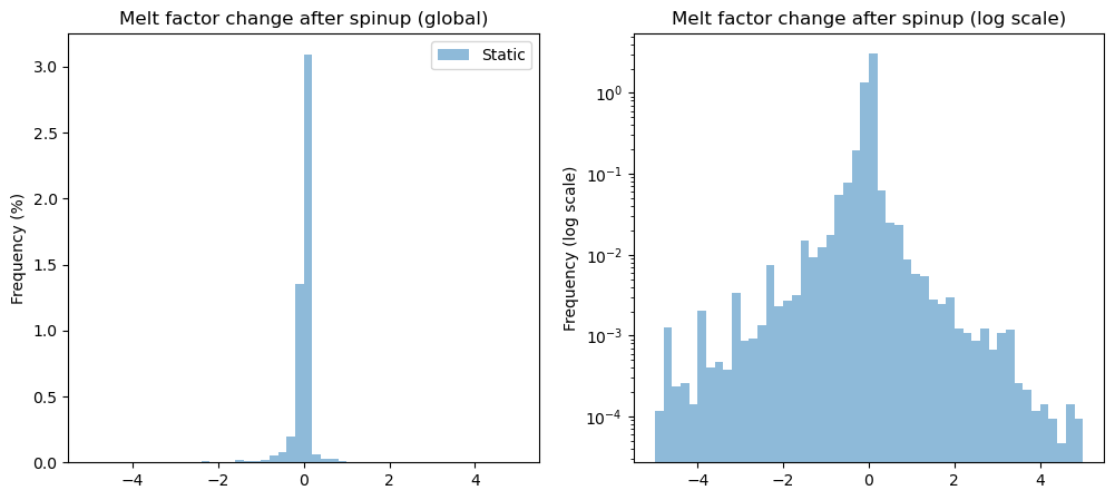
In which direction is the parameter changed?
diff = df_params['melt_f_dyna'] - df_params['melt_f']
f, (ax1, ax2) = plt.subplots(1, 2, figsize=(12, 5))
bins = np.linspace(-5, 5, 51)
diff.plot.hist(bins=bins, density=True, ax=ax1, alpha=0.5, label='Static');
ax1.set_title('Melt factor change after spinup (global)');
ax1.set_ylabel('Frequency (%)');
ax1.legend();

diff.plot.hist(bins=bins, density=True, ax=ax2, alpha=0.5, label='Static');
ax2.set_yscale('log')
ax2.set_title('Melt factor change after spinup (log scale)');
ax2.set_ylabel('Frequency (log scale)');
Take home#
dynamical spinup redistributes melt factors “for the best”, i.e. it increases a bit more the randomness of the melt factors around their central value
What’s next?#
return to the OGGM documentation
back to the table of contents