Ice thickness inversion

This example shows how to run the OGGM ice thickness inversion model with various ice parameters: the deformation parameter A and a sliding parameter (fs).

There is currently no “best” set of parameters for the ice thickness inversion model. As shown in Maussion et al. (2019), the default parameter set results in global volume estimates which are a bit larger than previous values. For the consensus estimate of Farinotti et al. (2019), OGGM participated with a deformation parameter A that is 1.5 times larger than the generally accepted default value.

There is no reason to think that the ice parameters are the same between neighboring glaciers. There is currently no “good” way to calibrate them, or at least no generaly accepted one. We won’t discuss the details here, but we provide a script to illustrate the sensitivity of the model to this choice.

New in version 1.4: we demonstrate how to apply a new global task in OGGM, workflow.calibrate_inversion_from_consensus to calibrate the A parameter to match the consensus estimate from Farinotti et al. (2019).

At the end of this tutorial, we show how to distribute the “flowline thicknesses” on a glacier map.

Run

# Libs
import geopandas as gpd

# Locals
import oggm.cfg as cfg
from oggm import utils, workflow, tasks, graphics

# Initialize OGGM and set up the default run parameters
cfg.initialize(logging_level='WARNING')
rgi_region = '11'  # Region Central Europe

# Local working directory (where OGGM will write its output)
WORKING_DIR = utils.gettempdir('OGGM_Inversion')
cfg.PATHS['working_dir'] = WORKING_DIR

# This is useful here
cfg.PARAMS['use_multiprocessing'] = True

# RGI file
path = utils.get_rgi_region_file(rgi_region)
rgidf = gpd.read_file(path)

# Select the glaciers in the Pyrenees
rgidf = rgidf.loc[rgidf['O2Region'] == '2']

# Sort for more efficient parallel computing
rgidf = rgidf.sort_values('Area', ascending=False)

# Go - get the pre-processed glacier directories
# We start at level 3, because we need all data for the inversion
# we need centerlines to use all functions of the distributed ice thickness later 
# (we specifically need `geometries.pkl` in the gdirs)
cfg.PARAMS['border'] = 80
base_url = ('https://cluster.klima.uni-bremen.de/~oggm/gdirs/oggm_v1.6/'
            'L3-L5_files/2023.3/centerlines/W5E5/')
gdirs = workflow.init_glacier_directories(rgidf, from_prepro_level=3,
                                         prepro_base_url=base_url)

# to assess the model geometry (for e.g. distributed ice thickness plots),
# we need to set that to true
#cfg.PARAMS['store_model_geometry'] = True
#workflow.execute_entity_task(tasks.prepare_for_inversion, gdirs)

# Default parameters
# Deformation: from Cuffey and Patterson 2010
glen_a = 2.4e-24
# Sliding: from Oerlemans 1997
fs = 5.7e-20

2024-04-25 13:29:42: oggm.cfg: Reading default parameters from the OGGM `params.cfg` configuration file.
2024-04-25 13:29:42: oggm.cfg: Multiprocessing switched OFF according to the parameter file.
2024-04-25 13:29:42: oggm.cfg: Multiprocessing: using all available processors (N=4)
2024-04-25 13:29:43: oggm.cfg: Multiprocessing switched ON after user settings.
2024-04-25 13:30:16: oggm.workflow: init_glacier_directories from prepro level 3 on 35 glaciers.
2024-04-25 13:30:16: oggm.workflow: Execute entity tasks [gdir_from_prepro] on 35 glaciers

with utils.DisableLogger():  # this scraps some output - to use with caution!!!
    
    # Correction factors
    factors = [0.1, 0.2, 0.3, 0.4, 0.5, 0.6, 0.7, 0.8, 0.9, 1]
    factors += [1.1, 1.2, 1.3, 1.5, 1.7, 2, 2.5, 3, 4, 5]
    factors += [6, 7, 8, 9, 10]

    # Run the inversions tasks with the given factors
    for f in factors:
        # Without sliding
        suf = '_{:03d}_without_fs'.format(int(f * 10))
        workflow.execute_entity_task(tasks.mass_conservation_inversion, gdirs,
                                     glen_a=glen_a*f, fs=0)
        # Store the results of the inversion only
        utils.compile_glacier_statistics(gdirs, filesuffix=suf,
                                         inversion_only=True)

        # With sliding
        suf = '_{:03d}_with_fs'.format(int(f * 10))
        workflow.execute_entity_task(tasks.mass_conservation_inversion, gdirs,
                                     glen_a=glen_a*f, fs=fs)
        # Store the results of the inversion only
        utils.compile_glacier_statistics(gdirs, filesuffix=suf,
                                         inversion_only=True)

Read the data

The data are stored as csv files in the working directory. The easiest way to read them is to use pandas!

import matplotlib.pyplot as plt
import pandas as pd
import numpy as np
from scipy import stats
import os

Let’s read the output of the inversion with the default OGGM parameters first:

df = pd.read_csv(os.path.join(WORKING_DIR, 'glacier_statistics_011_without_fs.csv'), index_col=0)
df

	rgi_region	rgi_subregion	name	cenlon	cenlat	rgi_area_km2	rgi_year	glacier_type	terminus_type	is_tidewater	...	vas_volume_km3	inv_volume_bsl_km3	inv_volume_bwl_km3	dem_source	n_orig_centerlines	flowline_type	perc_invalid_flowline	apparent_mb_from_any_mb_residual	inversion_glen_a	inversion_fs
rgi_id
RGI60-11.03208	11	11-02	Aneto	0.646032	42.641357	0.622	2011	Glacier	Land-terminating	False	...	0.017699	0.0	0.0	NASADEM	2	centerlines	0.205128	737.400000	2.640000e-24	0
RGI60-11.03232	11	11-02	Ossoue	-0.141222	42.771191	0.449	2011	Glacier	Land-terminating	False	...	0.011306	0.0	0.0	NASADEM	1	centerlines	0.000000	1168.200000	2.640000e-24	0
RGI60-11.03222	11	11-02	Monte Perdido Lower	0.039655	42.679337	0.308	2011	Glacier	Land-terminating	False	...	0.006733	0.0	0.0	NASADEM	2	centerlines	0.000000	887.700000	2.640000e-24	0
RGI60-11.03209	11	11-02	Maladeta E	0.639343	42.648979	0.260	2011	Glacier	Land-terminating	False	...	0.005334	0.0	0.0	NASADEM	1	centerlines	0.000000	593.500000	2.640000e-24	0
RGI60-11.03231	11	11-02	Oulettes Du Gaube	-0.144215	42.779716	0.130	2011	Glacier	Land-terminating	False	...	0.002057	0.0	0.0	NASADEM	1	centerlines	0.000000	509.400000	2.640000e-24	0
RGI60-11.03213	11	11-02	Seil De La Baque E	0.494304	42.694481	0.105	2011	Glacier	Land-terminating	False	...	0.001533	0.0	0.0	NASADEM	1	centerlines	0.000000	572.600000	2.640000e-24	0
RGI60-11.03239	11	11-02	Jezerces Gl No1	19.807627	42.465839	0.097	2007	Glacier	Land-terminating	False	...	0.001375	0.0	0.0	NASADEM	1	centerlines	0.562500	731.500000	2.640000e-24	0
RGI60-11.03229	11	11-02	Gabietous	-0.057456	42.695129	0.087	2011	Glacier	Land-terminating	False	...	0.001184	0.0	0.0	NASADEM	1	centerlines	0.000000	1600.600000	2.640000e-24	0
RGI60-11.03218	11	11-02	Llardana	0.428193	42.653946	0.084	2011	Glacier	Land-terminating	False	...	0.001128	0.0	0.0	NASADEM	1	centerlines	0.000000	1095.300000	2.640000e-24	0
RGI60-11.03228	11	11-02	Taillon	-0.039683	42.695419	0.083	2011	Glacier	Land-terminating	False	...	0.001110	0.0	0.0	NASADEM	1	centerlines	0.000000	1738.800000	2.640000e-24	0
RGI60-11.03205	11	11-02	Tempestades	0.666092	42.626839	0.077	2011	Glacier	Land-terminating	False	...	0.001001	0.0	0.0	NASADEM	1	centerlines	0.000000	108.800000	2.640000e-24	0
RGI60-11.03206	11	11-02	Barrancs	0.658785	42.632011	0.067	2011	Glacier	Land-terminating	False	...	0.000827	0.0	0.0	NASADEM	1	centerlines	0.000000	1392.800000	2.640000e-24	0
RGI60-11.03217	11	11-02	La Paul	0.437356	42.661072	0.057	2011	Glacier	Land-terminating	False	...	0.000662	0.0	0.0	NASADEM	1	centerlines	0.000000	882.900000	2.640000e-24	0
RGI60-11.03221	11	11-02	Monte Perdido Upper	0.033972	42.678589	0.054	2011	Glacier	Land-terminating	False	...	0.000614	0.0	0.0	NASADEM	1	centerlines	0.000000	871.000000	2.640000e-24	0
RGI60-11.03210	11	11-02	Maladeta W	0.632566	42.652107	0.054	2011	Glacier	Land-terminating	False	...	0.000614	0.0	0.0	NASADEM	1	centerlines	0.000000	402.100000	2.640000e-24	0
RGI60-11.03233	11	11-02	Infierno Central	-0.258849	42.783802	0.053	2011	Glacier	Land-terminating	False	...	0.000599	0.0	0.0	NASADEM	1	centerlines	0.000000	532.200000	2.640000e-24	0
RGI60-11.03225	11	11-02	Astazou	0.034118	42.703136	0.052	2011	Glacier	Land-terminating	False	...	0.000583	0.0	0.0	NASADEM	1	centerlines	0.000000	1260.300000	2.640000e-24	0
RGI60-11.03211	11	11-02	Boum	0.555278	42.700157	0.050	2011	Glacier	Land-terminating	False	...	0.000553	0.0	0.0	NASADEM	1	centerlines	0.000000	687.600000	2.640000e-24	0
RGI60-11.03240	11	11-02	Jezerces Gl No2	19.815450	42.447353	0.049	2007	Glacier	Land-terminating	False	...	0.000538	0.0	0.0	NASADEM	1	centerlines	0.000000	1706.700000	2.640000e-24	0
RGI60-11.03227	11	11-02	Pailla W	0.015287	42.705482	0.046	2011	Glacier	Land-terminating	False	...	0.000493	0.0	0.0	NASADEM	1	centerlines	0.000000	1058.400000	2.640000e-24	0
RGI60-11.03219	11	11-02	Barroude	0.142224	42.726147	0.042	2011	Glacier	Land-terminating	False	...	0.000435	0.0	0.0	NASADEM	1	centerlines	0.000000	620.000000	2.640000e-24	0
RGI60-11.03220	11	11-02	Munia	0.129816	42.717735	0.041	2011	Glacier	Land-terminating	False	...	0.000421	0.0	0.0	NASADEM	1	centerlines	0.000000	383.300000	2.640000e-24	0
RGI60-11.03212	11	11-02	Portillon D Oo	0.511460	42.693188	0.040	2011	Glacier	Land-terminating	False	...	0.000407	0.0	0.0	NASADEM	1	centerlines	0.000000	532.500000	2.640000e-24	0
RGI60-11.03226	11	11-02	Pailla E	0.021260	42.705322	0.035	2011	Glacier	Land-terminating	False	...	0.000339	0.0	0.0	NASADEM	1	centerlines	0.000000	-763.200000	2.640000e-24	0
RGI60-11.03241	11	11-02	It4L30000001 Gh Del Calderone	13.566710	42.470540	0.033	1990	Glacier	Land-terminating	False	...	0.000312	0.0	0.0	NASADEM	1	centerlines	0.250000	1036.800000	2.640000e-24	0
RGI60-11.03230	11	11-02	Petit Vignemale	-0.137718	42.775856	0.027	2011	Glacier	Land-terminating	False	...	0.000237	0.0	0.0	NASADEM	1	centerlines	0.000000	131.700000	2.640000e-24	0
RGI60-11.03215	11	11-02	Gourgs Blancs	0.480293	42.700859	0.026	2011	Glacier	Land-terminating	False	...	0.000225	0.0	0.0	NASADEM	1	centerlines	0.000000	677.300000	2.640000e-24	0
RGI60-11.03234	11	11-02	Las Neous	-0.286945	42.838642	0.025	2011	Glacier	Land-terminating	False	...	0.000213	0.0	0.0	NASADEM	1	centerlines	0.000000	346.200000	2.640000e-24	0
RGI60-11.03223	11	11-02	Marbore	0.018435	42.693417	0.023	2011	Glacier	Land-terminating	False	...	0.000190	0.0	0.0	NASADEM	1	centerlines	0.000000	596.371893	2.640000e-24	0
RGI60-11.03224	11	11-02	Cilindro	0.026603	42.689346	0.022	2011	Glacier	Land-terminating	False	...	0.000179	0.0	0.0	NASADEM	1	centerlines	0.000000	760.500000	2.640000e-24	0
RGI60-11.03204	11	11-02	Valier	1.088501	42.798626	0.021	2011	Glacier	Land-terminating	False	...	0.000168	0.0	0.0	NASADEM	1	centerlines	0.000000	596.371893	2.640000e-24	0
RGI60-11.03214	11	11-02	Seil De La Baque W	0.490498	42.696220	0.020	2011	Glacier	Land-terminating	False	...	0.000157	0.0	0.0	NASADEM	1	centerlines	0.000000	422.800000	2.640000e-24	0
RGI60-11.03238	11	11-02	Debeli Namet Gl	19.067500	43.115000	0.019	2003	Glacier	Land-terminating	False	...	0.000146	0.0	0.0	NASADEM	1	centerlines	0.000000	596.371893	2.640000e-24	0
RGI60-11.03207	11	11-02	Coronas	0.654112	42.632977	0.015	2011	Glacier	Land-terminating	False	...	0.000106	0.0	0.0	NASADEM	1	centerlines	0.000000	596.371893	2.640000e-24	0
RGI60-11.03216	11	11-02	Posets	0.438703	42.656570	0.010	2011	Glacier	Land-terminating	False	...	0.000060	0.0	0.0	NASADEM	1	centerlines	0.000000	596.371893	2.640000e-24	0

35 rows × 28 columns

There are only 35 glaciers in the Pyrenees! That’s why the run was relatively fast.

Results

One way to visualize the output is to plot the volume as a function of area in a log-log plot, illustrating the well known volume-area relationship of mountain glaciers:

ax = df.plot(kind='scatter', x='rgi_area_km2', y='inv_volume_km3')
ax.semilogx(); ax.semilogy()
xlim, ylim = [1e-2, 0.7], [1e-5, 0.05]
ax.set_xlim(xlim); ax.set_ylim(ylim);

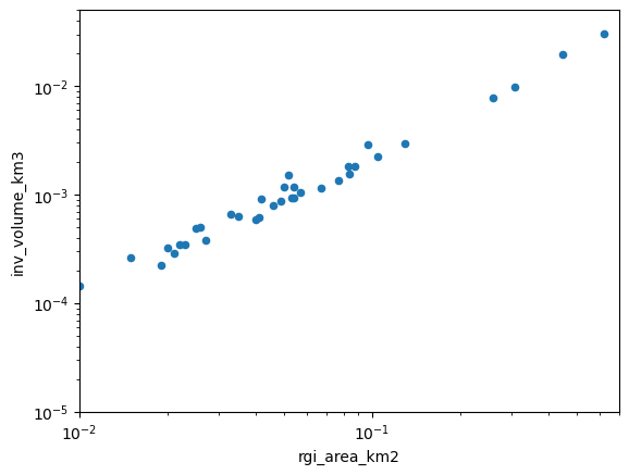
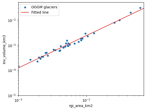
As we can see, there is a clear relationship, but it is not perfect. Let’s fit a line to these data (the “volume-area scaling law”):

# Fit in log space 
dfl = np.log(df[['inv_volume_km3', 'rgi_area_km2']])
slope, intercept, r_value, p_value, std_err = stats.linregress(dfl.rgi_area_km2.values, dfl.inv_volume_km3.values)

In their seminal paper, Bahr et al. (1997) describe this relationship as:

\[V = \alpha S^{\gamma}\]

With V the volume in km\(^3\), S the area in km\(^2\) and \(\alpha\) and \(\gamma\) the scaling parameters (0.034 and 1.375, respectively). How does OGGM compare to these in the Pyrenees?

print('power: {:.3f}'.format(slope))
print('slope: {:.3f}'.format(np.exp(intercept)))

power: 1.284
slope: 0.046

ax = df.plot(kind='scatter', x='rgi_area_km2', y='inv_volume_km3', label='OGGM glaciers')
ax.plot(xlim, np.exp(intercept) * (xlim ** slope), color='C3', label='Fitted line')
ax.semilogx(); ax.semilogy()
ax.set_xlim(xlim); ax.set_ylim(ylim);
ax.legend();

Sensitivity analysis

Now, let’s read the output files of each run separately, and compute the regional volume out of them:

dftot = pd.DataFrame(index=factors)
for f in factors:
    # Without sliding
    suf = '_{:03d}_without_fs'.format(int(f * 10))
    fpath = os.path.join(WORKING_DIR, 'glacier_statistics{}.csv'.format(suf))
    _df = pd.read_csv(fpath, index_col=0, low_memory=False)
    dftot.loc[f, 'without_sliding'] = _df.inv_volume_km3.sum()
    
    # With sliding
    suf = '_{:03d}_with_fs'.format(int(f * 10))
    fpath = os.path.join(WORKING_DIR, 'glacier_statistics{}.csv'.format(suf))
    _df = pd.read_csv(fpath, index_col=0, low_memory=False)
    dftot.loc[f, 'with_sliding'] = _df.inv_volume_km3.sum()

And plot them:

dftot.plot();
plt.xlabel('Factor of Glen A (default 1)'); plt.ylabel('Regional volume (km$^3$)');

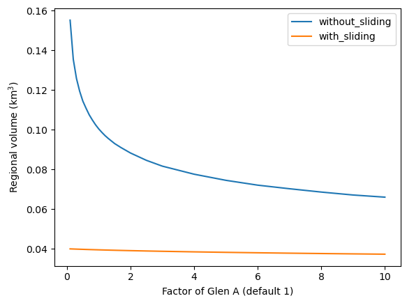
As you can see, there is quite a difference between the solutions. In particular, close to the default value for Glen A, the regional estimates are very sensitive to small changes in A. The calibration of A is a problem that has yet to be resolved by global glacier models…

Since OGGM version 1.4: calibrate to match the consensus estimate

Here, one “best Glen A” is found in order that the total inverted volume of the glaciers of gdirs fits to the 2019 consensus estimate.

# when we use all glaciers, no Glen A could be found within the range [0.1,10] that would match the consensus estimate
# usually, this is applied on larger regions where this error should not occur ! 
cdf = workflow.calibrate_inversion_from_consensus(gdirs[1:], filter_inversion_output=False)

2024-04-25 13:35:30: oggm.workflow: Applying global task calibrate_inversion_from_consensus on 34 glaciers
2024-04-25 13:35:30: oggm.workflow: Consensus estimate optimisation with A factor: 0.1 and fs: 0
2024-04-25 13:35:30: oggm.workflow: Applying global task inversion_tasks on 34 glaciers
2024-04-25 13:35:30: oggm.workflow: Execute entity tasks [prepare_for_inversion] on 34 glaciers
2024-04-25 13:35:30: oggm.workflow: Execute entity tasks [mass_conservation_inversion] on 34 glaciers
2024-04-25 13:35:30: oggm.workflow: Execute entity tasks [get_inversion_volume] on 34 glaciers
2024-04-25 13:35:30: oggm.workflow: Consensus estimate optimisation with A factor: 10.0 and fs: 0
2024-04-25 13:35:30: oggm.workflow: Applying global task inversion_tasks on 34 glaciers
2024-04-25 13:35:30: oggm.workflow: Execute entity tasks [prepare_for_inversion] on 34 glaciers
2024-04-25 13:35:30: oggm.workflow: Execute entity tasks [mass_conservation_inversion] on 34 glaciers
2024-04-25 13:35:30: oggm.workflow: Execute entity tasks [get_inversion_volume] on 34 glaciers
2024-04-25 13:35:30: oggm.workflow: Consensus estimate optimisation with A factor: 9.628954293399921 and fs: 0
2024-04-25 13:35:30: oggm.workflow: Applying global task inversion_tasks on 34 glaciers
2024-04-25 13:35:30: oggm.workflow: Execute entity tasks [prepare_for_inversion] on 34 glaciers
2024-04-25 13:35:30: oggm.workflow: Execute entity tasks [mass_conservation_inversion] on 34 glaciers
2024-04-25 13:35:30: oggm.workflow: Execute entity tasks [get_inversion_volume] on 34 glaciers
2024-04-25 13:35:30: oggm.workflow: Consensus estimate optimisation with A factor: 7.584273809665188 and fs: 0
2024-04-25 13:35:30: oggm.workflow: Applying global task inversion_tasks on 34 glaciers
2024-04-25 13:35:30: oggm.workflow: Execute entity tasks [prepare_for_inversion] on 34 glaciers
2024-04-25 13:35:30: oggm.workflow: Execute entity tasks [mass_conservation_inversion] on 34 glaciers
2024-04-25 13:35:30: oggm.workflow: Execute entity tasks [get_inversion_volume] on 34 glaciers
2024-04-25 13:35:30: oggm.workflow: Consensus estimate optimisation with A factor: 7.4100273087099495 and fs: 0
2024-04-25 13:35:30: oggm.workflow: Applying global task inversion_tasks on 34 glaciers
2024-04-25 13:35:30: oggm.workflow: Execute entity tasks [prepare_for_inversion] on 34 glaciers
2024-04-25 13:35:30: oggm.workflow: Execute entity tasks [mass_conservation_inversion] on 34 glaciers
2024-04-25 13:35:30: oggm.workflow: Execute entity tasks [get_inversion_volume] on 34 glaciers
2024-04-25 13:35:30: oggm.workflow: Consensus estimate optimisation with A factor: 7.3729771721654 and fs: 0
2024-04-25 13:35:30: oggm.workflow: Applying global task inversion_tasks on 34 glaciers
2024-04-25 13:35:30: oggm.workflow: Execute entity tasks [prepare_for_inversion] on 34 glaciers
2024-04-25 13:35:30: oggm.workflow: Execute entity tasks [mass_conservation_inversion] on 34 glaciers
2024-04-25 13:35:30: oggm.workflow: Execute entity tasks [get_inversion_volume] on 34 glaciers
2024-04-25 13:35:30: oggm.workflow: calibrate_inversion_from_consensus converged after 5 iterations and fs=0. The resulting Glen A factor is 7.4100273087099495.
2024-04-25 13:35:30: oggm.workflow: Applying global task inversion_tasks on 34 glaciers
2024-04-25 13:35:30: oggm.workflow: Execute entity tasks [prepare_for_inversion] on 34 glaciers
2024-04-25 13:35:30: oggm.workflow: Execute entity tasks [mass_conservation_inversion] on 34 glaciers
2024-04-25 13:35:30: oggm.workflow: Execute entity tasks [get_inversion_volume] on 34 glaciers

cdf.sum()

vol_itmix_m3        4.859110e+07
vol_bsl_itmix_m3    0.000000e+00
vol_oggm_m3         4.858508e+07
dtype: float64

Note that here we calibrate the Glen A parameter to a value that is equal for all glaciers of gdirs, i.e. we calibrate to match the total volume of all glaciers and not to match them individually.

cdf.iloc[:3]

	vol_itmix_m3	vol_bsl_itmix_m3	vol_oggm_m3
RGIId
RGI60-11.03232	1.422478e+07	0.0	1.380812e+07
RGI60-11.03222	5.158277e+06	0.0	7.253356e+06
RGI60-11.03209	5.335579e+06	0.0	5.483800e+06

just as a side note, “vol_bsl_itmix_m3” means volume below sea level and is therefore zero for these Alpine glaciers!

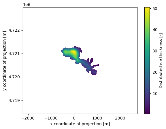
Distributed ice thickness

The OGGM inversion and dynamical models use the “1D” flowline assumption: for some applications, you might want to use OGGM to create distributed ice thickness maps. Currently, OGGM implements two ways to “distribute” the flowline thicknesses, but only the simplest one works robustly:

# Distribute
workflow.execute_entity_task(tasks.distribute_thickness_per_altitude, gdirs);

2024-04-25 13:35:30: oggm.workflow: Execute entity tasks [distribute_thickness_per_altitude] on 35 glaciers

We just created a new output of the model, which we can access in the gridded_data file:

# xarray is an awesome library! Did you know about it?
import xarray as xr
import rioxarray as rioxr
ds = xr.open_dataset(gdirs[0].get_filepath('gridded_data'))

ds.distributed_thickness.plot();

Since some people find geotiff data easier to read than netCDF, OGGM also provides a tool to convert the variables in gridded_data.nc file to a geotiff file:

# save the distributed ice thickness into a geotiff file
workflow.execute_entity_task(tasks.gridded_data_var_to_geotiff, gdirs, varname='distributed_thickness')

# The default path of the geotiff file is in the glacier directory with the name "distributed_thickness.tif"
# Let's check if the file exists
for gdir in gdirs:
    path = os.path.join(gdir.dir, 'distributed_thickness.tif')
    assert os.path.exists(path)

2024-04-25 13:35:32: oggm.workflow: Execute entity tasks [gridded_data_var_to_geotiff] on 35 glaciers

# Open the last file with xarray's open_rasterio
rioxr.open_rasterio(path).plot();

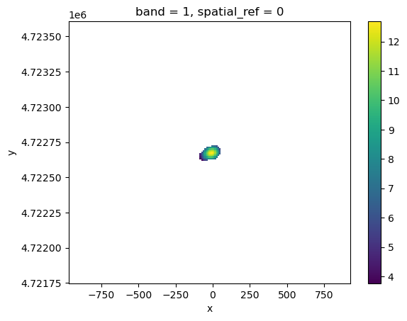
In fact, tasks.gridded_data_var_to_geotiff() can save any variable in the gridded_data.nc file. The geotiff is named as the variable name with a .tif suffix. Have a try by yourself ;-)

Plot many glaciers on a map

Let’s select a group of glaciers close to each other:

rgi_ids = ['RGI60-11.0{}'.format(i) for i in range(3205, 3211)]
sel_gdirs = [gdir for gdir in gdirs if gdir.rgi_id in rgi_ids]
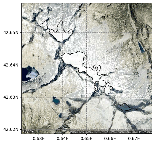
graphics.plot_googlemap(sel_gdirs)
# you might need to install motionless if it is not yet in your environment

Using OGGM

OGGM can plot the thickness of a group of glaciers on a map:

graphics.plot_distributed_thickness(sel_gdirs)

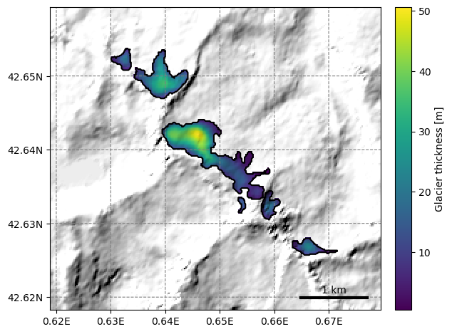
This is however not always very useful because OGGM can only plot on a map as large as the local glacier map of the first glacier in the list. See this issue for a discussion about why. In this case, we had a large enough border, and like that all neighboring glacers are visible.

Since this issue, several glaciers can be plotted at once by the kwarg extend_plot_limit=True:

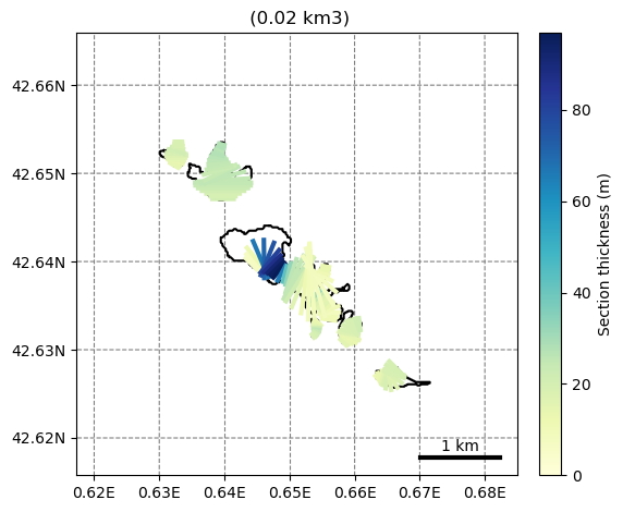
graphics.plot_inversion(sel_gdirs, extend_plot_limit=True)

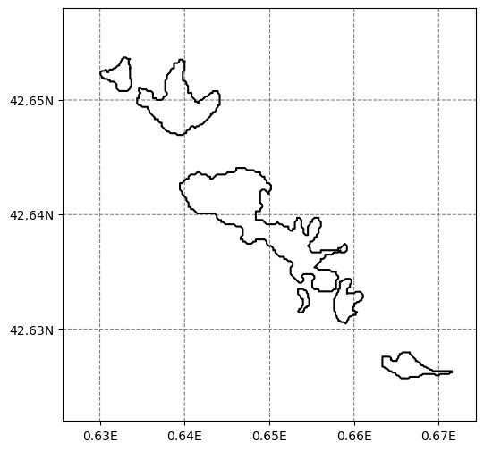
Using salem

Under the hood, OGGM uses salem to make the plots. Let’s do that for our case: it requires some manual tweaking, but it should be possible to automatize this better in the future.

Note: this also requires a version of salem after 21.05.2020

import salem
# Make a grid covering the desired map extent
g = salem.mercator_grid(center_ll=(0.65, 42.64), extent=(4000, 4000))
# Create a map out of it
smap = salem.Map(g, countries=False)
# Add the glaciers outlines
for gdir in sel_gdirs:
    crs = gdir.grid.center_grid
    geom = gdir.read_pickle('geometries')
    poly_pix = geom['polygon_pix']
    smap.set_geometry(poly_pix, crs=crs, fc='none', zorder=2, linewidth=.2)
    for l in poly_pix.interiors:
        smap.set_geometry(l, crs=crs, color='black', linewidth=0.5)
f, ax = plt.subplots(figsize=(6, 6))
smap.visualize();

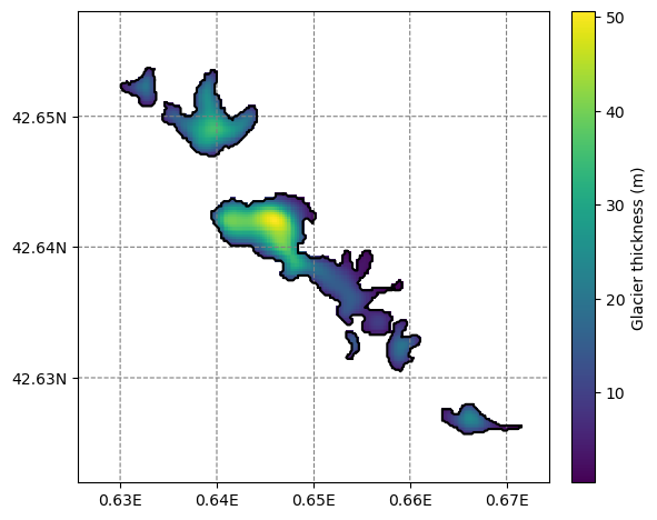
# Now add the thickness data
for gdir in sel_gdirs:
    grids_file = gdir.get_filepath('gridded_data')
    with utils.ncDataset(grids_file) as nc:
        vn = 'distributed_thickness'
        thick = nc.variables[vn][:]
        mask = nc.variables['glacier_mask'][:]
    thick = np.where(mask, thick, np.NaN)
    # The "overplot=True" is key here
    # this needs a recent version of salem to run properly
    smap.set_data(thick, crs=gdir.grid.center_grid, overplot=True)

# Set colorscale and other things
smap.set_cmap(graphics.OGGM_CMAPS['glacier_thickness'])
smap.set_plot_params(nlevels=256)
# Plot
f, ax = plt.subplots(figsize=(6, 6))
smap.visualize(ax=ax, cbar_title='Glacier thickness (m)');

What’s next?

• return to the OGGM documentation

• back to the table of contents