10 minutes to… OGGM as an accelerator for machine learning#
In this notebook, we want to showcase what OGGM does best: preparing data for your modelling workflow.
We use preprocessed directories which contain most data available in the OGGM shop to illustrate how these could be used to inform data-based workflows. The data that is available in the shop and is show cased here, is more than is required for the regular OGGM workflow, which you will see in a bit.
Tags: beginner, shop, workflow
Preprocessed directories with additional products#
We are going to use the South Glacier example taken from the ITMIX experiment. It is a small (5.6 km2) glacier in Alaska.
## Libs
import matplotlib.pyplot as plt
import numpy as np
import pandas as pd
import xarray as xr
import salem

# OGGM
import oggm.cfg as cfg
from oggm import utils, workflow, tasks, graphics
# Initialize OGGM and set up the default run parameters
cfg.initialize(logging_level='WARNING')
cfg.PARAMS['use_multiprocessing'] = False
# Local working directory (where OGGM will write its output)
cfg.PATHS['working_dir'] = utils.gettempdir('OGGM_Toy_Thickness_Model')
# We use the preprocessed directories with additional data in it: "W5E5_w_data"
base_url = 'https://cluster.klima.uni-bremen.de/~oggm/gdirs/oggm_v1.6/L3-L5_files/2023.3/elev_bands/W5E5_w_data/'
gdirs = workflow.init_glacier_directories(['RGI60-01.16195'], from_prepro_level=3, prepro_base_url=base_url, prepro_border=10)
2024-04-25 13:13:10: oggm.cfg: Reading default parameters from the OGGM `params.cfg` configuration file.
2024-04-25 13:13:10: oggm.cfg: Multiprocessing switched OFF according to the parameter file.
2024-04-25 13:13:10: oggm.cfg: Multiprocessing: using all available processors (N=4)
2024-04-25 13:13:12: oggm.workflow: init_glacier_directories from prepro level 3 on 1 glaciers.
2024-04-25 13:13:12: oggm.workflow: Execute entity tasks [gdir_from_prepro] on 1 glaciers
# Pick our glacier
gdir = gdirs[0]
gdir
<oggm.GlacierDirectory>
  RGI id: RGI60-01.16195
  Region: 01: Alaska
  Subregion: 01-05: St Elias Mtns
  Glacier type: Glacier
  Terminus type: Land-terminating
  Status: Glacier or ice cap
  Area: 5.655 km2
  Lon, Lat: (-139.131, 60.822)
  Grid (nx, ny): (105, 121)
  Grid (dx, dy): (43.0, -43.0)
OGGM-Shop datasets#
We are using here the preprocessed glacier directories that contain more data than the default ones:
with xr.open_dataset(gdir.get_filepath('gridded_data')) as ds:
    ds = ds.load()
# List all variables
ds
<xarray.Dataset> Size: 598kB
Dimensions:                  (x: 105, y: 121)
Coordinates:
  * x                        (x) float32 420B -2.407e+03 ... 2.065e+03
  * y                        (y) float32 484B 6.746e+06 6.745e+06 ... 6.74e+06
Data variables: (12/14)
    topo                     (y, x) float32 51kB 2.5e+03 2.505e+03 ... 2.118e+03
    topo_smoothed            (y, x) float32 51kB 2.507e+03 ... 2.137e+03
    topo_valid_mask          (y, x) int8 13kB 1 1 1 1 1 1 1 1 ... 1 1 1 1 1 1 1
    glacier_mask             (y, x) int8 13kB 0 0 0 0 0 0 0 0 ... 0 0 0 0 0 0 0
    glacier_ext              (y, x) int8 13kB 0 0 0 0 0 0 0 0 ... 0 0 0 0 0 0 0
    consensus_ice_thickness  (y, x) float32 51kB nan nan nan nan ... nan nan nan
    ...                       ...
    itslive_v                (y, x) float32 51kB 33.22 30.73 ... 0.8565 1.049
    millan_ice_thickness     (y, x) float32 51kB 172.7 175.0 177.4 ... nan nan
    millan_v                 (y, x) float32 51kB 43.39 40.9 38.69 ... 0.0 0.0
    millan_vx                (y, x) float32 51kB -27.17 -25.96 ... 0.0 0.0
    millan_vy                (y, x) float32 51kB 33.84 31.61 28.85 ... 0.0 0.0
    hugonnet_dhdt            (y, x) float32 51kB -0.3103 -0.2804 ... -0.02641
Attributes:
    author:         OGGM
    author_info:    Open Global Glacier Model
    pyproj_srs:     +proj=tmerc +lat_0=0 +lon_0=-139.131 +k=0.9996 +x_0=0 +y_...
    max_h_dem:      3158.8242
    min_h_dem:      1804.8026
    max_h_glacier:  3158.8242
min_h_glacier: 1971.5164That’s already quite a lot! We have access to a bunch of data for this glacier, lets have a look. We prepare the map first:
smap = ds.salem.get_map(countries=False)
smap.set_shapefile(gdir.read_shapefile('outlines'))
smap.set_topography(ds.topo.data);
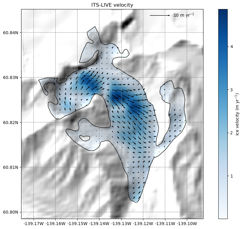
ITSLive velocity data#
Lets start with the ITSLIVE velocity data:
# get the velocity data
u = ds.itslive_vx.where(ds.glacier_mask)
v = ds.itslive_vy.where(ds.glacier_mask)
ws = ds.itslive_v.where(ds.glacier_mask)
The .where(ds.glacier_mask) command will remove the data outside of the glacier outline.
# get the axes ready
f, ax = plt.subplots(figsize=(9, 9))
# Quiver only every N grid point
us = u[1::3, 1::3]
vs = v[1::3, 1::3]
smap.set_data(ws)
smap.set_cmap('Blues')
smap.plot(ax=ax)
smap.append_colorbar(ax=ax, label='ice velocity (m yr$^{-1}$)')
# transform their coordinates to the map reference system and plot the arrows
xx, yy = smap.grid.transform(us.x.values, us.y.values, crs=gdir.grid.proj)
xx, yy = np.meshgrid(xx, yy)
qu = ax.quiver(xx, yy, us.values, vs.values)
qk = ax.quiverkey(qu, 0.82, 0.97, 10, '10 m yr$^{-1}$',
labelpos='E', coordinates='axes')
ax.set_title('ITS-LIVE velocity');
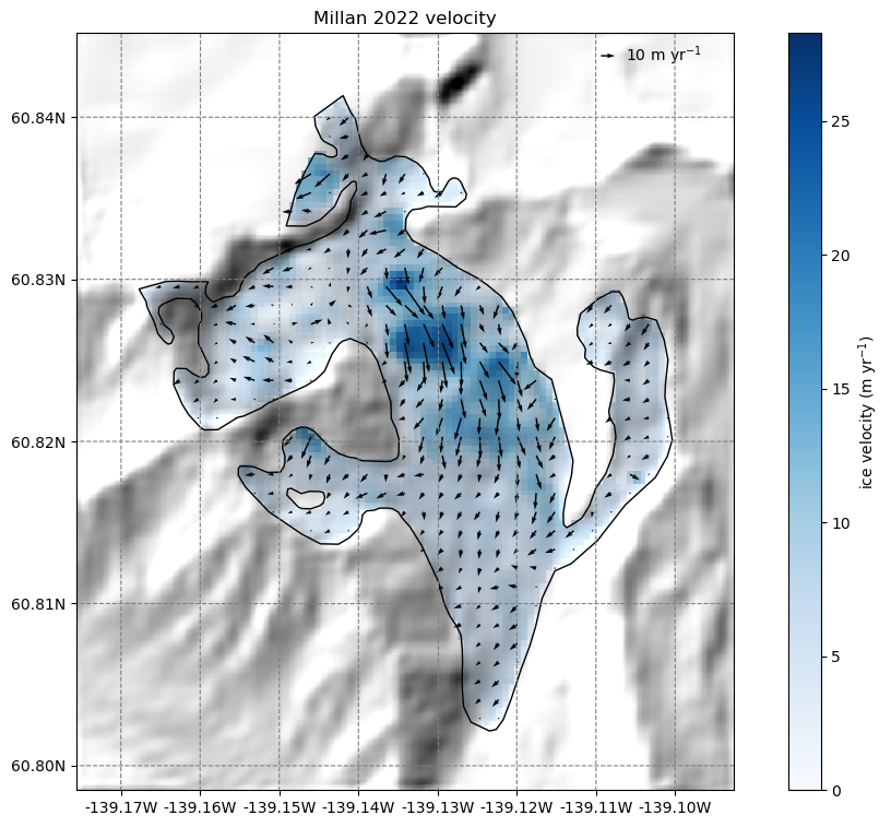
Millan 2022 velocity data#
There is more velocity data. Here follows the Millan et al. (2022) dataset:
# get the velocity data
u = ds.millan_vx.where(ds.glacier_mask)
v = ds.millan_vy.where(ds.glacier_mask)
ws = ds.millan_v.where(ds.glacier_mask)
# get the axes ready
f, ax = plt.subplots(figsize=(9, 9))
# Quiver only every N grid point
us = u[1::3, 1::3]
vs = v[1::3, 1::3]
smap.set_data(ws)
smap.set_cmap('Blues')
smap.plot(ax=ax)
smap.append_colorbar(ax=ax, label='ice velocity (m yr$^{-1}$)')
# transform their coordinates to the map reference system and plot the arrows
xx, yy = smap.grid.transform(us.x.values, us.y.values, crs=gdir.grid.proj)
xx, yy = np.meshgrid(xx, yy)
qu = ax.quiver(xx, yy, us.values, vs.values)
qk = ax.quiverkey(qu, 0.82, 0.97, 10, '10 m yr$^{-1}$',
labelpos='E', coordinates='axes')
ax.set_title('Millan 2022 velocity');
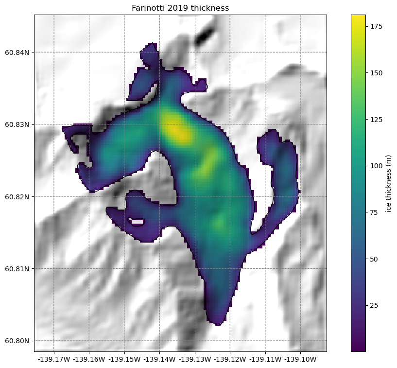
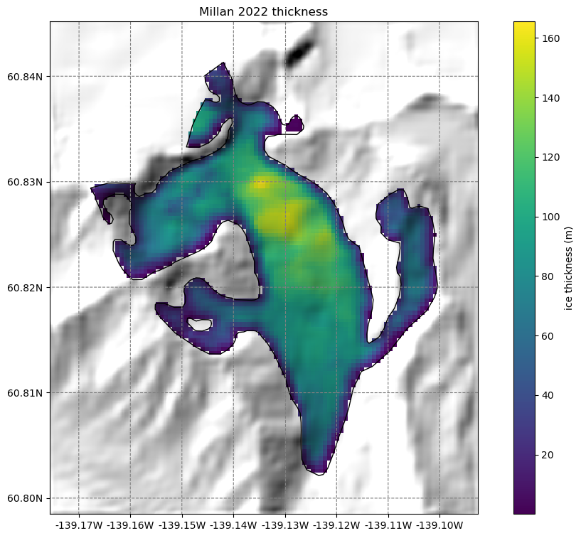
Thickness data from Farinotti 2019 and Millan 2022#
We also provide ice thickness data from Farinotti et al. (2019) and Millan et al. (2022) in the same gridded format.
# get the axes ready
f, ax = plt.subplots(figsize=(9, 9))
smap.set_cmap('viridis')
smap.set_data(ds.consensus_ice_thickness)
smap.plot(ax=ax)
smap.append_colorbar(ax=ax, label='ice thickness (m)')
ax.set_title('Farinotti 2019 thickness');
# get the axes ready
f, ax = plt.subplots(figsize=(9, 9))
smap.set_cmap('viridis')
smap.set_data(ds.millan_ice_thickness.where(ds.glacier_mask))
smap.plot(ax=ax)
smap.append_colorbar(ax=ax, label='ice thickness (m)')
ax.set_title('Millan 2022 thickness');
Some additional gridded attributes#
Let’s also add some attributes that OGGM can compute for us:
# Tested tasks
task_list = [
tasks.gridded_attributes,
tasks.gridded_mb_attributes,
]
for task in task_list:
workflow.execute_entity_task(task, gdirs)
2024-04-25 13:13:27: oggm.workflow: Execute entity tasks [gridded_attributes] on 1 glaciers
2024-04-25 13:13:27: oggm.workflow: Execute entity tasks [gridded_mb_attributes] on 1 glaciers
Let’s open the gridded data file again with xarray:
with xr.open_dataset(gdir.get_filepath('gridded_data')) as ds:
ds = ds.load()
# List all variables
ds
<xarray.Dataset> Size: 979kB
Dimensions: (x: 105, y: 121)
Coordinates:
* x (x) float32 420B -2.407e+03 ... 2.065e+03
* y (y) float32 484B 6.746e+06 6.745e+06 ... 6.74e+06
Data variables: (12/23)
topo (y, x) float32 51kB 2.5e+03 2.505e+03 ... 2.118e+03
topo_smoothed (y, x) float32 51kB 2.507e+03 ... 2.137e+03
topo_valid_mask (y, x) int8 13kB 1 1 1 1 1 1 1 1 ... 1 1 1 1 1 1 1
glacier_mask (y, x) int8 13kB 0 0 0 0 0 0 0 0 ... 0 0 0 0 0 0 0
glacier_ext (y, x) int8 13kB 0 0 0 0 0 0 0 0 ... 0 0 0 0 0 0 0
consensus_ice_thickness (y, x) float32 51kB nan nan nan nan ... nan nan nan
... ...
aspect (y, x) float32 51kB 5.777 5.66 ... 1.788 1.874
slope_factor (y, x) float32 51kB 3.872 3.872 ... 2.571 3.092
dis_from_border (y, x) float32 51kB 1.727e+03 ... 1.632e+03
catchment_area (y, x) float32 51kB nan nan nan nan ... nan nan nan
lin_mb_above_z (y, x) float32 51kB nan nan nan nan ... nan nan nan
oggm_mb_above_z (y, x) float32 51kB nan nan nan nan ... nan nan nan
Attributes:
author: OGGM
author_info: Open Global Glacier Model
pyproj_srs: +proj=tmerc +lat_0=0 +lon_0=-139.131 +k=0.9996 +x_0=0 +y_...
max_h_dem: 3158.8242
min_h_dem: 1804.8026
max_h_glacier: 3158.8242
min_h_glacier: 1971.5164The file contains several new variables with their description. For example:
ds.oggm_mb_above_z
<xarray.DataArray 'oggm_mb_above_z' (y: 121, x: 105)> Size: 51kB
array([[nan, nan, nan, ..., nan, nan, nan],
       [nan, nan, nan, ..., nan, nan, nan],
       [nan, nan, nan, ..., nan, nan, nan],
       ...,
       [nan, nan, nan, ..., nan, nan, nan],
       [nan, nan, nan, ..., nan, nan, nan],
       [nan, nan, nan, ..., nan, nan, nan]], dtype=float32)
Coordinates:
* x (x) float32 420B -2.407e+03 -2.364e+03 ... 2.022e+03 2.065e+03
* y (y) float32 484B 6.746e+06 6.745e+06 ... 6.74e+06 6.74e+06
Attributes:
units: kg/year
long_name: MB above point from OGGM MB model, without catchments
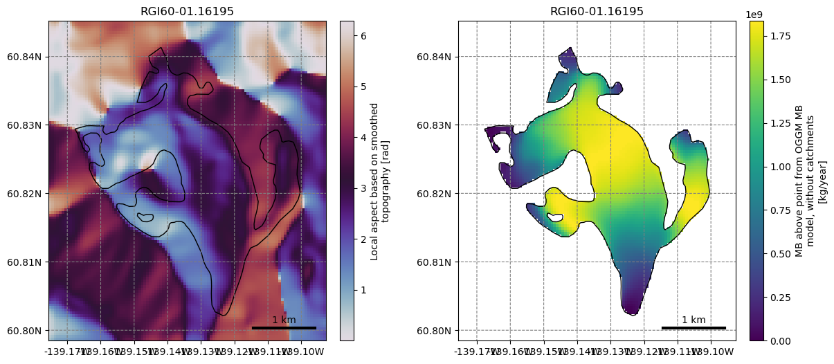
description: Mass balance cumulated above the altitude of thepoint, henc...Let’s plot a few of them (we show how to plot them with xarray and with oggm):
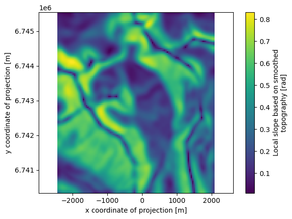
ds.slope.plot();
plt.axis('equal');
f, (ax1, ax2) = plt.subplots(1, 2, figsize=(14, 6))
graphics.plot_raster(gdir, var_name='aspect', cmap='twilight', ax=ax1)
graphics.plot_raster(gdir, var_name='oggm_mb_above_z', ax=ax2)
Not convinced yet? Lets spend 10 more minutes to apply a (very simple) machine learning workflow#
Retrieve these attributes at point locations#
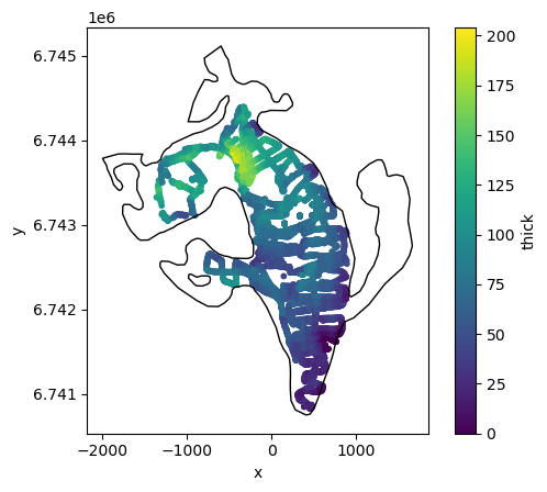
For this glacier, we have ice thickness observations (all downloaded from the supplementary material of the ITMIX paper). Let’s make a table out of it:
df = salem.read_shapefile(utils.get_demo_file('IceThick_SouthGlacier.shp'))
coords = np.array([p.xy for p in df.geometry]).squeeze()
df['lon'] = coords[:, 0]
df['lat'] = coords[:, 1]
df = df[['lon', 'lat', 'thick']]
Convert the longitudes and latitudes to the glacier map projection:
xx, yy = salem.transform_proj(salem.wgs84, gdir.grid.proj, df['lon'].values, df['lat'].values)
df['x'] = xx
df['y'] = yy
And plot these data:
geom = gdir.read_shapefile('outlines')
f, ax = plt.subplots()
df.plot.scatter(x='x', y='y', c='thick', cmap='viridis', s=10, ax=ax);
geom.plot(ax=ax, facecolor='none', edgecolor='k');
Method 1: interpolation#
The measurement points of this dataset are very frequent and close to each other. There are plenty of them:
len(df)
9619
Here, we will keep them all and interpolate the variables of interest at the point’s location. We use xarray for this:
vns = ['topo',
       'slope',
       'slope_factor',
       'aspect',
       'dis_from_border',
       'catchment_area',
       'lin_mb_above_z',
       'oggm_mb_above_z',
       'millan_v',
       'itslive_v',
       ]
# Interpolate (bilinear)
for vn in vns:
    df[vn] = ds[vn].interp(x=('z', df.x), y=('z', df.y))
Let’s see how these variables can explain the measured ice thickness:
f, (ax1, ax2, ax3) = plt.subplots(1, 3, figsize=(16, 5))
df.plot.scatter(x='dis_from_border', y='thick', ax=ax1); ax1.set_title('dis_from_border');
df.plot.scatter(x='slope', y='thick', ax=ax2); ax2.set_title('slope');
df.plot.scatter(x='oggm_mb_above_z', y='thick', ax=ax3); ax3.set_title('oggm_mb_above_z');
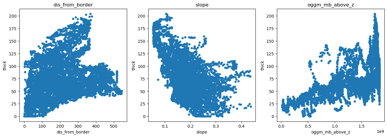
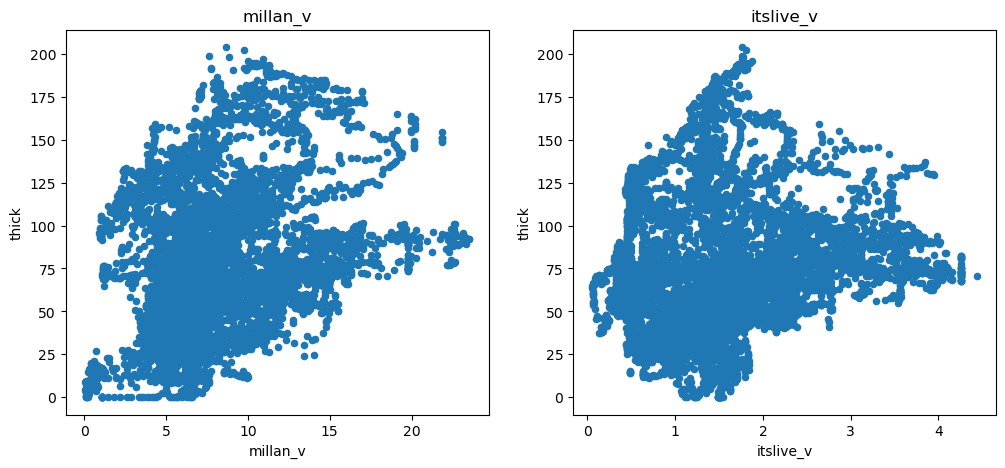
There is a negative correlation with slope (as expected), a positive correlation with the mass-flux (oggm_mb_above_z), and a slight positive correlation with the distance from the glacier boundaries. There is also some correlaction with ice velocity, but not a strong one:
f, (ax1, ax2) = plt.subplots(1, 2, figsize=(12, 5))
df.plot.scatter(x='millan_v', y='thick', ax=ax1); ax1.set_title('millan_v');
df.plot.scatter(x='itslive_v', y='thick', ax=ax2); ax2.set_title('itslive_v');
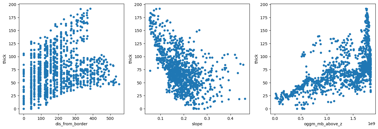
Method 2: aggregated per grid point#
There are so many points that much of the information obtained by OGGM is interpolated and therefore not biring much new information to a statistical model. A way to deal with this is to aggregate all the measurement points per grid point and to average them. Let’s do this:
df_agg = df[['lon', 'lat', 'thick']].copy()
ii, jj = gdir.grid.transform(df['lon'], df['lat'], crs=salem.wgs84, nearest=True)
df_agg['i'] = ii
df_agg['j'] = jj
# We trick by creating an index of similar i's and j's
df_agg['ij'] = ['{:04d}_{:04d}'.format(i, j) for i, j in zip(ii, jj)]
df_agg = df_agg.groupby('ij').mean()
# Conversion does not preserve ints
df_agg['i'] = df_agg['i'].astype(int)
df_agg['j'] = df_agg['j'].astype(int)
len(df_agg)
1087
# Select
for vn in vns:
    df_agg[vn] = ds[vn].isel(x=('z', df_agg['i']), y=('z', df_agg['j']))
We now have 9 times less points, but the main features of the data remain unchanged:
f, (ax1, ax2, ax3) = plt.subplots(1, 3, figsize=(16, 5))
df_agg.plot.scatter(x='dis_from_border', y='thick', ax=ax1);
df_agg.plot.scatter(x='slope', y='thick', ax=ax2);
df_agg.plot.scatter(x='oggm_mb_above_z', y='thick', ax=ax3);
Build a statistical model#
Let’s use scikit-learn to build a very simple linear model of ice-thickness. First, we have to acknowledge that there is a correlation between many of the explanatory variables we will use:
import seaborn as sns
plt.figure(figsize=(10, 8));
sns.heatmap(df.corr(), cmap='RdBu');
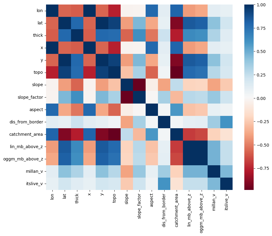
This is a problem for linear regression models, which cannot deal well with correlated explanatory variables. We have to do a so-called “feature selection”, i.e. keep only the variables which are independently important to explain the outcome.
For the sake of simplicity, let’s use the Lasso method to help us out:
import warnings
warnings.filterwarnings("ignore")  # sklearn sends a lot of warnings
# Scikit learn (can be installed e.g. via conda install -c anaconda scikit-learn)
from sklearn.linear_model import LassoCV
from sklearn.model_selection import KFold
# Prepare our data
df = df.dropna()
# Variable to model
target = df['thick']
# Predictors - remove x and y (redundant with lon lat)
# Normalize it in order to be able to compare the factors
data = df.drop(['thick', 'x', 'y'], axis=1).copy()
data_mean = data.mean()
data_std = data.std()
data = (data - data_mean) / data_std
# Use cross-validation to select the regularization parameter
lasso_cv = LassoCV(cv=5, random_state=0)
lasso_cv.fit(data.values, target.values)
LassoCV(cv=5, random_state=0)In a Jupyter environment, please rerun this cell to show the HTML representation or trust the notebook.
On GitHub, the HTML representation is unable to render, please try loading this page with nbviewer.org.
LassoCV(cv=5, random_state=0)
We now have a statistical model trained on the full dataset. Let’s see how it compares to the calibration data:
odf = df.copy()
odf['thick_predicted'] = lasso_cv.predict(data.values)
f, ax = plt.subplots(figsize=(6, 6));
odf.plot.scatter(x='thick', y='thick_predicted', ax=ax);
plt.xlim([-25, 220]);
plt.ylim([-25, 220]);
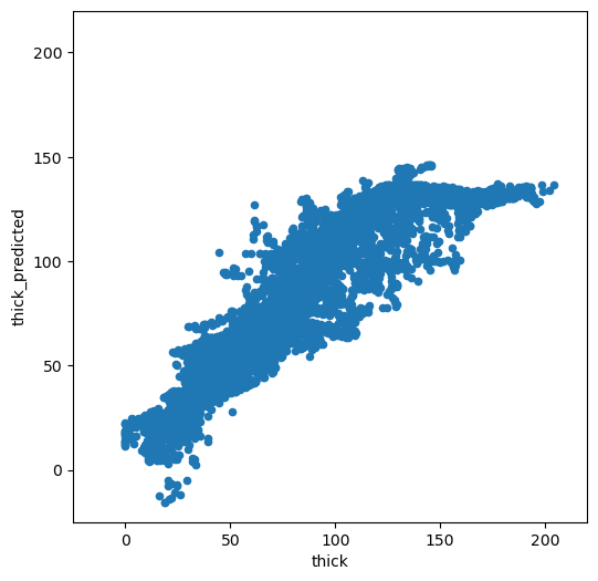
Not too bad. It is doing OK for low thicknesses, but high thickness are strongly underestimated. Which explanatory variables did the model choose as being the most important?
predictors = pd.Series(lasso_cv.coef_, index=data.columns)
predictors
lon                -6.483752
lat                13.074533
topo                0.000000
slope              -0.000000
slope_factor       14.529238
aspect             -7.133175
dis_from_border     1.469916
catchment_area     -0.000000
lin_mb_above_z      2.223419
oggm_mb_above_z     0.000000
millan_v            0.000000
itslive_v          -0.000000
dtype: float64
This is interesting. Lons and lats have a predictive power over thickness? Unfortunately, this is more a coincidence than a reality. If we look at the correlation of the error with the variables of importance, one sees that there is a large correlation between the error and the spatial variables:
odf['error'] = np.abs(odf['thick_predicted'] - odf['thick'])
odf.corr()['error'].loc[predictors.loc[predictors != 0].index]
lon               -0.320308
lat                0.379959
slope_factor       0.278369
aspect            -0.182406
dis_from_border    0.023982
lin_mb_above_z     0.260073
Name: error, dtype: float64
Furthermore, the model is not very robust. Let’s use cross-validation to check our model parameters:
k_fold = KFold(4, random_state=0, shuffle=True)
for k, (train, test) in enumerate(k_fold.split(data.values, target.values)):
    lasso_cv.fit(data.values[train], target.values[train])
    print("[fold {0}] alpha: {1:.5f}, score (r^2): {2:.5f}".
          format(k, lasso_cv.alpha_, lasso_cv.score(data.values[test], target.values[test])))
[fold 0] alpha: 1.45567, score (r^2): 0.80985
[fold 1] alpha: 1.57309, score (r^2): 0.81848
[fold 2] alpha: 1.35209, score (r^2): 0.80951
[fold 3] alpha: 1.44635, score (r^2): 0.81532
The fact that the hyper-parameter alpha and the score change that much between iterations is a sign that the model isn’t very robust.
Our model is not great, but… let’s apply it#
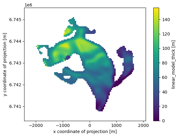
In order to apply the model to our entre glacier, we have to get the explanatory variables from the gridded dataset again:
# Add variables we are missing
lon, lat = gdir.grid.ll_coordinates
ds['lon'] = (('y', 'x'), lon)
ds['lat'] = (('y', 'x'), lat)

# Generate our dataset
pred_data = pd.DataFrame()
for vn in data.columns:
    pred_data[vn] = ds[vn].data[ds.glacier_mask == 1]

# Normalize using the same normalization constants
pred_data = (pred_data - data_mean) / data_std

# Apply the model
pred_data['thick'] = lasso_cv.predict(pred_data.values)

# For the sake of physics, clip negative thickness values...
pred_data['thick'] = np.clip(pred_data['thick'], 0, None)
# Back to 2d and in xarray
var = ds[vn].data * np.NaN
var[ds.glacier_mask == 1] = pred_data['thick']
ds['linear_model_thick'] = (('y', 'x'), var)
ds['linear_model_thick'].attrs['description'] = 'Predicted thickness'
ds['linear_model_thick'].attrs['units'] = 'm'
ds['linear_model_thick'].plot();
Take home points#
OGGM provides preprocessed data from different sources on the same grid
we have shown how to compute gridded attributes from OGGM glaciers such as slope, aspect, or catchments
we used two methods to extract these data at point locations: with interpolation or with aggregated averages on each grid point
as an application example, we trained a linear regression model to predict the ice thickness of this glacier at unseen locations
The model we developed was quite bad and we used quite lousy statistics. If I had more time to make it better, I would:
make a pre-selection of meaningful predictors to avoid discontinuities
use a non-linear model
use cross-validation to better asses the true skill of the model
…
What’s next?#
return to the OGGM documentation
back to the table of contents
Bonus: how does the statistical model compare to OGGM “out-of the box” and other thickness products?#
# Write our thinckness estimates back to disk
ds.to_netcdf(gdir.get_filepath('gridded_data'))
# Distribute OGGM thickness using default values only
workflow.execute_entity_task(tasks.distribute_thickness_per_altitude, gdirs);
2024-04-25 13:13:34: oggm.workflow: Execute entity tasks [distribute_thickness_per_altitude] on 1 glaciers
with xr.open_dataset(gdir.get_filepath('gridded_data')) as ds:
    ds = ds.load()
df_agg['oggm_thick'] = ds.distributed_thickness.isel(x=('z', df_agg['i']), y=('z', df_agg['j']))
df_agg['linear_model_thick'] = ds.linear_model_thick.isel(x=('z', df_agg['i']), y=('z', df_agg['j']))
df_agg['millan_thick'] = ds.millan_ice_thickness.isel(x=('z', df_agg['i']), y=('z', df_agg['j']))
df_agg['consensus_thick'] = ds.consensus_ice_thickness.isel(x=('z', df_agg['i']), y=('z', df_agg['j']))
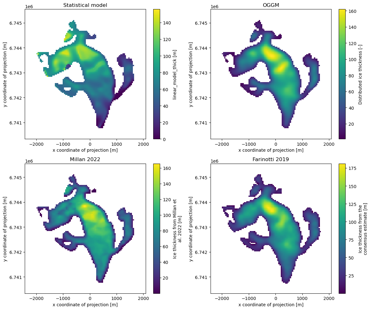
f, ((ax1, ax2), (ax3, ax4)) = plt.subplots(2, 2, figsize=(12, 10));
ds['linear_model_thick'].plot(ax=ax1); ax1.set_title('Statistical model');
ds['distributed_thickness'].plot(ax=ax2); ax2.set_title('OGGM');
ds['millan_ice_thickness'].where(ds.glacier_mask).plot(ax=ax3); ax3.set_title('Millan 2022');
ds['consensus_ice_thickness'].plot(ax=ax4); ax4.set_title('Farinotti 2019');
plt.tight_layout();
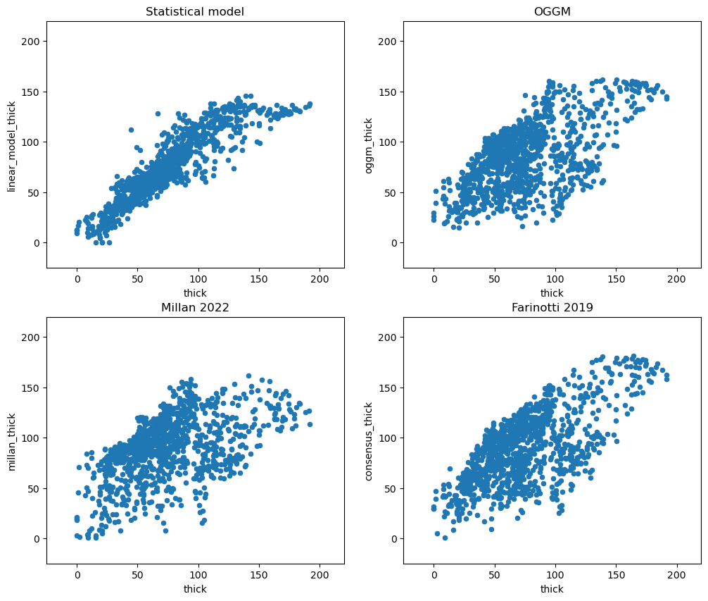
f, ((ax1, ax2), (ax3, ax4)) = plt.subplots(2, 2, figsize=(12, 10));
df_agg.plot.scatter(x='thick', y='linear_model_thick', ax=ax1);
ax1.set_xlim([-25, 220]); ax1.set_ylim([-25, 220]); ax1.set_title('Statistical model');
df_agg.plot.scatter(x='thick', y='oggm_thick', ax=ax2);
ax2.set_xlim([-25, 220]); ax2.set_ylim([-25, 220]); ax2.set_title('OGGM');
df_agg.plot.scatter(x='thick', y='millan_thick', ax=ax3);
ax3.set_xlim([-25, 220]); ax3.set_ylim([-25, 220]); ax3.set_title('Millan 2022');
df_agg.plot.scatter(x='thick', y='consensus_thick', ax=ax4);
ax4.set_xlim([-25, 220]); ax4.set_ylim([-25, 220]); ax4.set_title('Farinotti 2019');