Merge, analyse and visualize OGGM GCM runs

Merge, analyse and visualize OGGM GCM runs#

In this notebook we want to show:

How to merge the output of different OGGM GCM projections into one dataset
How to calculate regional values (e.g. volume) using the merged dataset
How to use matplotlib or seaborn to visualize the projections and plot different statistical estimates (median, interquartile range, mean, std, …)
How to use HoloViews and Panel to visualize the outcome. This part uses advanced plotting capabilities which are not necessary to understand the rest of the notebook.

This notebook is intended to explain the postprocessing steps, rather than the OGGM workflow itself. Therefore some code (especially conducting the GCM projection runs) does not have many explanations. If you are more interested in these steps you should check out the notebook Run OGGM with GCM data.

GCM projection runs#

The first step is to conduct the GCM projection runs. We choose two different glaciers by their rgi_ids and conduct the GCM projections. Again if you do not understand all of the following code you should check out the Run OGGM with GCM data notebook.

# Libs
from time import gmtime, strftime
import xarray as xr
import numpy as np

# Locals
from oggm import utils, workflow, tasks, DEFAULT_BASE_URL
import oggm.cfg as cfg
from oggm.shop import gcm_climate

Pre-processed directories#

# Initialize OGGM and set up the default run parameters
cfg.initialize(logging_level='WARNING')

# change border around the individual glaciers
cfg.PARAMS['border'] = 80

# Use Multiprocessing
cfg.PARAMS['use_multiprocessing'] = True

# For hydro output
cfg.PARAMS['store_model_geometry'] = True

# Local working directory (where OGGM will write its output)
cfg.PATHS['working_dir'] = utils.gettempdir('OGGM_merge_gcm_runs', reset=True)

# RGI glaciers: Ngojumba and Khumbu
rgi_ids = utils.get_rgi_glacier_entities(['RGI60-15.03473', 'RGI60-15.03733'])

# Go - get the pre-processed glacier directories
# in OGGM v1.6 you have to explicitly indicate the url from where you want to start from
# we will use here the elevation band flowlines which are much simpler than the centerlines
gdirs = workflow.init_glacier_directories(rgi_ids, from_prepro_level=5, prepro_base_url=DEFAULT_BASE_URL)

2024-04-25 13:38:03: oggm.cfg: Reading default parameters from the OGGM `params.cfg` configuration file.
2024-04-25 13:38:03: oggm.cfg: Multiprocessing switched OFF according to the parameter file.
2024-04-25 13:38:03: oggm.cfg: Multiprocessing: using all available processors (N=4)
2024-04-25 13:38:04: oggm.cfg: Multiprocessing switched ON after user settings.
2024-04-25 13:38:04: oggm.cfg: PARAMS['store_model_geometry'] changed from `False` to `True`.
2024-04-25 13:38:10: oggm.workflow: init_glacier_directories from prepro level 5 on 2 glaciers.
2024-04-25 13:38:10: oggm.workflow: Execute entity tasks [gdir_from_prepro] on 2 glaciers

Download and process GCM data#

In this notebook, we will use the bias-corrected ISIMIP3b GCM files. You can also use directly CMIP5 or CMIP6 (how to do that is explained in run_with_gcm).

all_GCM = ['gfdl-esm4_r1i1p1f1', 'ipsl-cm6a-lr_r1i1p1f1',
           'mpi-esm1-2-hr_r1i1p1f1',
           'mri-esm2-0_r1i1p1f1', 'ukesm1-0-ll_r1i1p1f2']

# define the SSP scenarios
all_scenario = ['ssp126', 'ssp370', 'ssp585']

for GCM in all_GCM:
    for ssp in all_scenario:
        # we will pretend that 'mpi-esm1-2-hr_r1i1p1f1' is missing for `ssp370`
        # to later show how to deal with missing values, 
        # if you want to use this
        # code you can of course remove the "if" and just download all GCMs and SSPS 
        if (ssp == 'ssp370') & (GCM=='mpi-esm1-2-hr_r1i1p1f1'):
            pass
        else:
            # Download and process them:
            workflow.execute_entity_task(gcm_climate.process_monthly_isimip_data, gdirs, 
                                         ssp = ssp,
                                         # gcm ensemble -> you can choose another one
                                         member=GCM,
                                         # recognize the climate file for later
                                         output_filesuffix=f'_{GCM}_{ssp}'
                                         );
            
# you could create a similar workflow with CMIP5 or CMIP6 

2024-04-25 13:38:10: oggm.workflow: Execute entity tasks [process_monthly_isimip_data] on 2 glaciers
2024-04-25 13:38:23: oggm.workflow: Execute entity tasks [process_monthly_isimip_data] on 2 glaciers
2024-04-25 13:38:30: oggm.workflow: Execute entity tasks [process_monthly_isimip_data] on 2 glaciers
2024-04-25 13:38:36: oggm.workflow: Execute entity tasks [process_monthly_isimip_data] on 2 glaciers
2024-04-25 13:38:49: oggm.workflow: Execute entity tasks [process_monthly_isimip_data] on 2 glaciers
2024-04-25 13:38:55: oggm.workflow: Execute entity tasks [process_monthly_isimip_data] on 2 glaciers
2024-04-25 13:39:01: oggm.workflow: Execute entity tasks [process_monthly_isimip_data] on 2 glaciers
2024-04-25 13:39:14: oggm.workflow: Execute entity tasks [process_monthly_isimip_data] on 2 glaciers
2024-04-25 13:39:20: oggm.workflow: Execute entity tasks [process_monthly_isimip_data] on 2 glaciers
2024-04-25 13:39:21: oggm.workflow: Execute entity tasks [process_monthly_isimip_data] on 2 glaciers
2024-04-25 13:39:22: oggm.workflow: Execute entity tasks [process_monthly_isimip_data] on 2 glaciers
2024-04-25 13:39:23: oggm.workflow: Execute entity tasks [process_monthly_isimip_data] on 2 glaciers
2024-04-25 13:39:36: oggm.workflow: Execute entity tasks [process_monthly_isimip_data] on 2 glaciers
2024-04-25 13:39:42: oggm.workflow: Execute entity tasks [process_monthly_isimip_data] on 2 glaciers

Here we defined, downloaded and processed all the GCM models and scenarios (here 5 GCMs and three SSPs). We pretend that one GCM is missing for one scenario (this is sometimes the case in for example CMIP5 GCMs, see e.g. this table). We deal with possible missing GCMs for specific SCENARIOs by by including a try/except in the code below and by taking care that the missing values are filled with NaN values (and stay NaN when doing sums).

Actual projection Runs#

Now we conduct the actual projection runs. Again handling the case that for a certain (GCM, SCENARIO) combination no data is available with a try/except.

for GCM in all_GCM:
    for scen in all_scenario:
        rid = '_{}_{}'.format(GCM, scen)
        try:  # check if (GCM, scen) combination exists
            workflow.execute_entity_task(tasks.run_with_hydro, gdirs,
                                         run_task=tasks.run_from_climate_data,
                                         ys=2020,  # star year of our projection runs
                                         climate_filename='gcm_data',  # use gcm_data, not climate_historical
                                         climate_input_filesuffix=rid,  # use the chosen GCM and scenario
                                         init_model_filesuffix='_spinup_historical',  # this is important! Start from 2020 glacier
                                         output_filesuffix=rid,  # the filesuffix of the resulting file, so we can find it later
                                         store_monthly_hydro=True
                                        );

        except FileNotFoundError:
            # if a certain scenario is not available for a GCM we land here
            # and we inidcate this by printing a message so the user knows
            # this scenario is missing
            # (in this case of course, the file actually is available, but we just pretend that it is not...)
            print('No ' + GCM +' run with scenario ' + scen + ' available!')

No mpi-esm1-2-hr_r1i1p1f1 run with scenario ssp370 available!

2024-04-25 13:39:48: oggm.workflow: Execute entity tasks [run_with_hydro] on 2 glaciers
2024-04-25 13:39:49: oggm.workflow: Execute entity tasks [run_with_hydro] on 2 glaciers
2024-04-25 13:39:50: oggm.workflow: Execute entity tasks [run_with_hydro] on 2 glaciers
2024-04-25 13:39:51: oggm.workflow: Execute entity tasks [run_with_hydro] on 2 glaciers
2024-04-25 13:39:52: oggm.workflow: Execute entity tasks [run_with_hydro] on 2 glaciers
2024-04-25 13:39:53: oggm.workflow: Execute entity tasks [run_with_hydro] on 2 glaciers
2024-04-25 13:39:54: oggm.workflow: Execute entity tasks [run_with_hydro] on 2 glaciers
2024-04-25 13:39:55: oggm.workflow: Execute entity tasks [run_with_hydro] on 2 glaciers
2024-04-25 13:39:55: oggm.workflow: Execute entity tasks [run_with_hydro] on 2 glaciers
2024-04-25 13:39:56: oggm.workflow: Execute entity tasks [run_with_hydro] on 2 glaciers
2024-04-25 13:39:56: oggm.workflow: Execute entity tasks [run_with_hydro] on 2 glaciers
2024-04-25 13:39:57: oggm.workflow: Execute entity tasks [run_with_hydro] on 2 glaciers
2024-04-25 13:39:58: oggm.workflow: Execute entity tasks [run_with_hydro] on 2 glaciers
2024-04-25 13:39:59: oggm.workflow: Execute entity tasks [run_with_hydro] on 2 glaciers
2024-04-25 13:40:00: oggm.workflow: Execute entity tasks [run_with_hydro] on 2 glaciers

Visualisation with matplotlib or seaborn#

We will first use matplotlib, where we need to estimate the statistical estimates ourselves. This is good to understand what we are doing.

import matplotlib.pyplot as plt

# estimate the minimum volume for each time step and scenario over the GCMs
ds_total_volume_min = ds_total_volume.min(dim='GCM', keep_attrs=True,skipna=True)
# estimate the 25th percentile volume for each time step and scenario over the GCMs
ds_total_volume_p25 = ds_total_volume.quantile(0.25, dim='GCM', keep_attrs=True,skipna=True)
# estimate the 50th percentile volume for each time step and scenario over the GCMs
ds_total_volume_p50 = ds_total_volume.quantile(0.5, dim='GCM', keep_attrs=True,skipna=True)
# this is the same as the median -> Let's check
np.testing.assert_allclose(ds_total_volume_median,ds_total_volume_p50)
# estimate the 75th percentile volume for each time step and scenario over the GCMs
ds_total_volume_p75 = ds_total_volume.quantile(0.75, dim='GCM', keep_attrs=True,skipna=True)
# estimate the maximum volume for each time step and scenario over the GCMs
ds_total_volume_max = ds_total_volume.max(dim='GCM', keep_attrs=True,skipna=True)

# Think twice if it is appropriate to compute a mean/std over your GCM sample, is it Gaussian distributed?
# Otherwise use instead median and percentiles or total range
ds_total_volume_mean = ds_total_volume.mean(dim='GCM', keep_attrs=True,
                                            skipna=True)
ds_total_volume_std = ds_total_volume.std(dim='GCM', keep_attrs=True,
                                            skipna=True)

color_dict={'ssp126':'blue', 'ssp370':'orange', 'ssp585':'red'}


fig, axs = plt.subplots(1,2, figsize=(12,6), 
                        sharey=True # we want to share the y axis betweeen the subplots
                       )
for scenario in color_dict.keys():
    # get amount of GCMs per Scenario to add it to the legend:
    n = len(ds_total_volume.sel(SCENARIO=scenario).dropna(dim='GCM').GCM)
    axs[0].plot(ds_total_volume_median.time,
                ds_total_volume_median.sel(SCENARIO=scenario)/1e9,  # m3 -> km3
                label=f'{scenario}: n={n} GCMs',
                color=color_dict[scenario],lw=3)
    axs[0].fill_between(ds_total_volume_median.time,
                        ds_total_volume_p25.sel(SCENARIO=scenario)/1e9,
                        ds_total_volume_p75.sel(SCENARIO=scenario)/1e9,
                        color=color_dict[scenario],
                        alpha=0.5,
                        label='interquartile range\n(75th-25th percentile)')
    axs[0].fill_between(ds_total_volume_median.time,
                        ds_total_volume_min.sel(SCENARIO=scenario)/1e9,
                        ds_total_volume_max.sel(SCENARIO=scenario)/1e9,
                        color=color_dict[scenario],
                        alpha=0.1,
                        label='total range')


for scenario in color_dict.keys():
    axs[1].plot(ds_total_volume_mean.time,
                 ds_total_volume_mean.sel(SCENARIO=scenario)/1e9,  # m3 -> km3
                 color=color_dict[scenario],
                 label='mean',lw=3)
    axs[1].fill_between(ds_total_volume_mean.time,
                        ds_total_volume_mean.sel(SCENARIO=scenario)/1e9 - ds_total_volume_std.sel(SCENARIO=scenario)/1e9,
                        ds_total_volume_mean.sel(SCENARIO=scenario)/1e9 + ds_total_volume_std.sel(SCENARIO=scenario)/1e9,
                        alpha=0.3,
                        color=color_dict[scenario],
                       label='standard deviation')
    
for ax in axs:
    # get all handles and labels and then create two different legends
    handles, labels = ax.get_legend_handles_labels()
    if ax == axs[0]:
        # we want to have two legends, let's save the first one
        # which just shows the colors and the different SSPs here 
        leg1 = ax.legend(handles[:3], labels[:3], title='Scenario') 
        ax.set_ylabel(r'Volume (km$^3$)')
        # create the second one, that shows the different statistical estimates
        ax.legend([handles[0],handles[3],handles[4]],
                  ['median',labels[3],labels[4]], loc='lower left')
        # we need to allow for two legend, this is done like that
        ax.add_artist(leg1)
    else:
        # for the second plot, we only want to have the legend for mean and std
        ax.legend(handles[::3], labels[::3], loc='lower left') 
    ax.set_xlabel('Year');
    ax.grid()

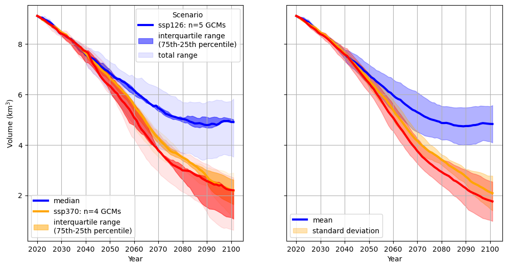
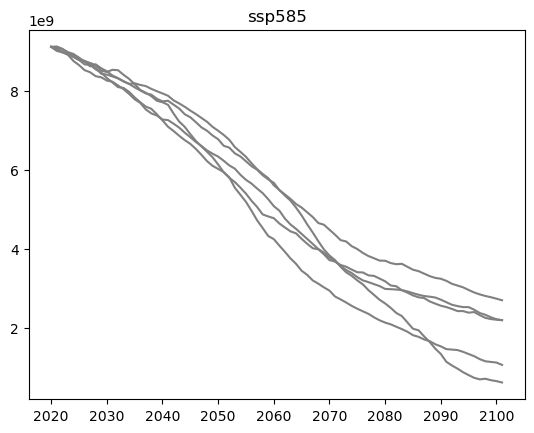
../../_images/40404f83286c4c6bf09757cb1cab678714d8212c42b150f06a1a75ce468cca1b.png

You have to choose which statistical estimate is best in your case. It is also a good possibility to just plot all the scenarios, and then to decide which statistical estimate describes best the spread in your case:

# for example, if there are just 5 GCMs, maybe you can just show all of them?
for gcm in all_GCM: 
    plt.plot(ds_total_volume.sel(SCENARIO=scenario).time,
            ds_total_volume.sel(SCENARIO=scenario, GCM=gcm),
             color='grey')
plt.title(scenario)

Text(0.5, 1.0, 'ssp585')

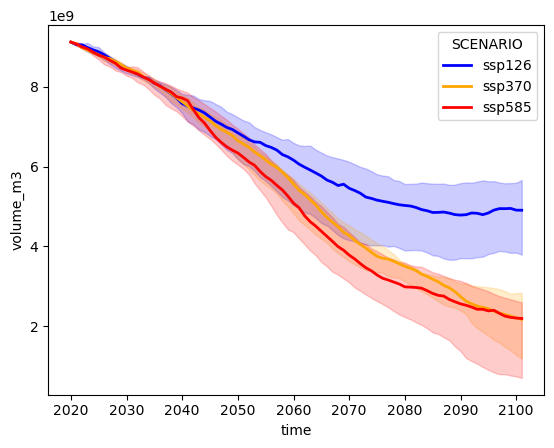
../../_images/cfa2de4b0bf47ebaa36c95b3ef687b7625406c595d591bae668aa37d52265272.png

You could create similar plots even easier with seaborn, which has a lot of statistical estimation tools directly included (specifically in seaborn>=v0.12). You can for example check out this errorbar seaborn tutorial. Note that the outcome can be slightly different even for the same statistical estimate as e.g. seaborn and xarray might use different methods to compute the same thing.

import seaborn as sns 
# this code might only work with seaborn v>=0.12
# seaborn always likes to have pandas dataframes
pd_total_volume = ds_total_volume.to_dataframe('volume_m3').reset_index()
sns.lineplot(x='time', y='volume_m3',
             hue='SCENARIO', # these are the dimension for the different colors 
             estimator='median', # here you could also choose the mean
             data=pd_total_volume,
             lw=2, # increase the linewidth a bit
             palette= color_dict, # let's use the same colors as before
             # for errorbar you could also choose another percentile range
             # see: https://seaborn.pydata.org/tutorial/error_bars.html
             # "90" means the range goes from the 5th to the 95th percentile
             # (50 would be the interquartile range, i.e., the same as two plots above)
             errorbar=('pi', 90) 
            );

../../_images/a5ceb53bea63e29824e0ebc4bc961dcab8c091e3cec9288d2f6d81c48cfa6005.png

Interactive visualisation with HoloViews and Panel#

the following code only works if you install holoviews and panel

We can also visualize the data using tools from the HoloViz framework (namely HoloViews and Panel). For an introduction to HoloViz, you can have a look at the Small overview of HoloViz capability of data exploration notebook.

# Plotting
import holoviews as hv
import panel as pn
hv.extension('bokeh')
pn.extension()

To make your life easier with Holoviews and Panel, you can define a small function that computes your estimates:

In the following section, we only show mean and std, but this could be similar applied to the median and specific percentiles (which might be more robust in your use case :-) ). But just for showing how it works, it is fine to use here mean and std!

def calculate_total_mean_and_std(ds, variable):
    mean = ds[variable].sum(dim='rgi_id',  # first sum up over all glaciers
                            skipna=True,
                            keep_attrs=True,
                            # important, need values for every glacier
                            min_count=len(ds_merged.rgi_id), 
                           ).mean(dim='GCM',  # afterwards calculate the mean of all GCMs
                                  skipna=True,
                                  keep_attrs=True,
                                 )
    std = ds[variable].sum(dim='rgi_id',  # first sum up over all glaciers 
                           skipna=True,
                           keep_attrs=True,
                           min_count=len(ds_merged.rgi_id), 
                          ).std(dim='GCM',  # afterwards calculate the std of all GCMs
                                skipna=True,
                                keep_attrs=True,
                               )
    return mean, std

This function takes a dataset ds and a variable name variable for which the mean and the std should be calculated. This function will come in handy in the next section dealing with the visualisation of the calculated values.

First, we create a single curve for a single scenario (here ssp585):

# calculate mean and std with the previously defined function
total_volume_mean, total_volume_std = calculate_total_mean_and_std(ds_merged, 'volume')

# select only one SSP scenario
total_volume_mean_ssp585 = total_volume_mean.loc[{'SCENARIO': 'ssp585'}]

# plot a curve
x = total_volume_mean_ssp585.coords['time']
y = total_volume_mean_ssp585
hv.Curve((x, y),
         kdims=x.name,
         vdims=y.name,
        ).opts(xlabel=x.attrs['description'],
               ylabel=f"{y.attrs['description']} in {y.attrs['unit']}")

We used a HoloViews Curve and defined kdims and vdims. This definition is not so important for a single plot but if we start to compose different plots all axis of the different plots with the same kdims or vdims are connected. This means for example whenever you zoom in on one plot all other plots also zoom in. Further, you can see that we have defined xlabel and ylabel using the variable description of the dataset, therefore it was useful to keep_attrs=True when we calculated the total values (see above).

As a next step we can add the std as a shaded area (HoloViews Area) and again define the whole plot as a single curve in a new function:

Create single mean curve with std area#

def get_single_curve(mean, std, ssp):
    color = color_dict[ssp] 
    mean_use = mean.loc[{'SCENARIO': ssp}]  # read out the mean of the SSP to plot 
    std_use = std.loc[{'SCENARIO': ssp}]  # read out the std of the SSP to plot
    time = mean.coords['time']  # get the time for the x axis
    
    return (hv.Area((time,  # plot std as an area
                     mean_use + std_use,  # upper boundary of the area
                     mean_use - std_use),  # lower boundary of the area
                    vdims=[mean_use.name, 'y2'],  # vdims for both boundaries
                    kdims='time',
                    label=ssp,
                   ).opts(alpha=0.2,
                          line_color=None,
                         ) *
            hv.Curve((time, mean_use),
                     vdims=mean_use.name,
                     kdims='time',
                     label=ssp,
                     
                    ).opts(line_color=color)
           ).opts(width=400,  # width of the total plot
                  height=400,  # height of the total plot
                  xlabel=time.attrs['description'],
                  ylabel=f"{mean_use.attrs['description']} in {mean_use.attrs['unit']}",
                 )

Overlay different scenarios#

The single curves of the different scenarios we can put together in a HoloViews HoloMap, which is comparable to a dictionary. This further can be easily used to create a nice overlay of all curves.

def overlay_scenarios(ds, variable):
    hmap = hv.HoloMap(kdims='Scenarios')   # create a HoloMap
    mean, std = calculate_total_mean_and_std(ds, variable)  # calculate mean and std for all SSPs using our previously defined function
    for ssp in all_scenario:
        hmap[ssp] = get_single_curve(mean, std, ssp)  # add a curve for each SSP to the HoloMap, using the SSP as a key (when you compare it do a dictonary)
    return hmap.overlay().opts(title=variable)  # create an overlay of all curves

Show different variables in one figure and save as html file#

Now that we have defined how our plots should look like we can compose different variables we want to explore in one plot. To do so we can use Panel Column and Row for customization of the plot layout:

all_plots = pn.Column(pn.Row(overlay_scenarios(ds_merged, 'volume'),
                             overlay_scenarios(ds_merged, 'area'),
                            ),
                      overlay_scenarios(ds_merged, 'melt_on_glacier'))

all_plots

When you start exploring the plots by dragging them around or zooming in (using the tools of the toolboxes in the upper right corner of each plot) you see that the x-axes are connected. This makes it very convenient for example to look at different periods for all variables interactively.

You also can open the plots in a new browser tab by using

all_plots.show()

or save it as a html file for sharing

plots_to_save = pn.panel(all_plots)
plots_to_save.save('GCM_runs.html', embed=True)

What’s next?#

return to the OGGM documentation
back to the table of contents