What’s in my preprocessed directories with centerlines? A full OGGM workflow, step by step#
The OGGM workflow is best explained with an example. In the following, we will show how to apply the standard OGGM workflow to a list of glaciers. This example is meant to guide you through a first-time setup step-by-step. If you prefer not to install OGGM on your computer, you can always run this notebook in OGGM-Edu instead!
Set-up#
Input data folders#
If you are using your own computer: before you start, make sure that you have set-up the input data configuration file at your wish.
In the course of this tutorial, we will need to download data needed for each glacier (a couple of mb at max, depending on the chosen glaciers), so make sure you have an internet connection.
cfg.initialize() and cfg.PARAMS#
An OGGM simulation script will always start with the following commands:
from oggm import cfg, utils
cfg.initialize(logging_level='WARNING')
2024-04-25 13:23:42: oggm.cfg: Reading default parameters from the OGGM `params.cfg` configuration file.
2024-04-25 13:23:42: oggm.cfg: Multiprocessing switched OFF according to the parameter file.
2024-04-25 13:23:42: oggm.cfg: Multiprocessing: using all available processors (N=4)
A call to cfg.initialize() will read the default parameter file (or any user-provided file) and make them available to all other OGGM tools via the cfg.PARAMS dictionary. Here are some examples of these parameters:
cfg.PARAMS['melt_f'], cfg.PARAMS['ice_density'], cfg.PARAMS['continue_on_error']
(5.0, 900.0, False)
See here for the default parameter file and a description of their role and default value.
# You can try with or without multiprocessing: with two glaciers, OGGM could run on two processors
cfg.PARAMS['use_multiprocessing'] = True
2024-04-25 13:23:43: oggm.cfg: Multiprocessing switched ON after user settings.
Workflow#
In this section, we will explain the fundamental concepts of the OGGM workflow:
Working directories
Glacier directories
Tasks
from oggm import workflow
Working directory#
Each OGGM run needs a single folder where to store the results of the computations for all glaciers. This is called a “working directory” and needs to be specified before each run. Here we create a temporary folder for you:
cfg.PATHS['working_dir'] = utils.gettempdir(dirname='OGGM-GettingStarted', reset=True)
cfg.PATHS['working_dir']
'/tmp/OGGM/OGGM-GettingStarted'
We use a temporary directory for this example, but in practice you will set this working directory yourself (for example: /home/john/OGGM_output. The size of this directory will depend on how many glaciers you’ll simulate!
This working directory is meant to be persistent, i.e. you can stop your processing workflow after any task, and restart from an existing working directory at a later stage.
You can create a persistent OGGM working directory at a specific path via path = utils.mkdir(path). Beware! If you use reset=True in utils.mkdir, ALL DATA in this folder will be deleted! Use it with caution!
Define the glaciers for the run#
rgi_ids = ['RGI60-11.01328', 'RGI60-11.00897']
You can provide any number of glacier identifiers to OGGM. In this case, we chose:
RGI60-11.01328: Unteraar Glacier in the Swiss AlpsRGI60-11.00897: Hintereisferner in the Austrian Alps.
Here is a list of other glaciers you might want to try out:
RGI60-18.02342: Tasman Glacier in New ZealandRGI60-11.00787: Kesselwandferner in the Austrian Alps… or any other glacier identifier! You can find other glacier identifiers by exploring the GLIMS viewer.
For an operational run on an RGI region, you might want to download the Randolph Glacier Inventory dataset instead, and start a run from it. This case is covered in the working with the RGI tutorial.
Glacier directories#
The OGGM workflow is organized as a list of tasks that have to be applied to a list of glaciers. The vast majority of tasks are called entity tasks: they are standalone operations to be realized on one single glacier entity. These tasks are executed sequentially (one after another): they often need input generated by the previous task(s): for example, the climate calibration needs the glacier flowlines, which can be only computed after the topography data has been processed, and so on.
To handle this situation, OGGM uses a workflow based on data persistence on disk: instead of passing data as python variables from one task to another, each task will read the data from disk and then write the computation results back to the disk, making these new data available for the next task in the queue.
These glacier specific data are located in glacier directories. In the model, these directories are initialized with the following command (this can take a little while on the first call, as OGGM needs to download some data):
# Where to fetch the pre-processed directories
base_url = 'https://cluster.klima.uni-bremen.de/~oggm/gdirs/oggm_v1.6/L3-L5_files/2023.3/centerlines/W5E5'
gdirs = workflow.init_glacier_directories(rgi_ids, from_prepro_level=3, prepro_base_url=base_url, prepro_border=80)
2024-04-25 13:23:44: oggm.workflow: init_glacier_directories from prepro level 3 on 2 glaciers.
2024-04-25 13:23:44: oggm.workflow: Execute entity tasks [gdir_from_prepro] on 2 glaciers
the keyword
from_prepro_levelindicates that we will start from pre-processed directories, i.e. data that are already pre-processed for the model users. In many cases you will want to start from level 3, 4 or 5. Here we start from level 3 and rerun some of the processing in order to demonstrate the OGGM workflow.the
prepro_borderkeyword indicates the number of DEM grid points which we’d like to add to each side of the glacier for the local map: the larger the glacier will grow, the larger the border parameter should be. The available pre-processed border values are: 10, 80, 160 (depending on the model set-ups there might be more or less options). These are the fixed map sizes we prepared for you - any other map size will require a full processing (see the alternative DEM example for a tutorial).
The init_glacier_directories task will allways be the very first task to call for all your OGGM experiments. Let’s see what it gives us back:
type(gdirs), type(gdirs[0])
(list, oggm.utils._workflow.GlacierDirectory)
gdirs is a list of GlacierDirectory objects (one for each glacier). Glacier directories are used by OGGM as “file and attribute manager” for single glaciers. For example, the model now knows where to find the topography data file for this glacier:
gdir = gdirs[0]  # take Unteraar glacier
print('Path to the DEM:', gdir.get_filepath('dem'))
Path to the DEM: /tmp/OGGM/OGGM-GettingStarted/per_glacier/RGI60-11/RGI60-11.01/RGI60-11.01328/dem.tif
And we can also access some attributes of this glacier:
gdir
<oggm.GlacierDirectory>
  RGI id: RGI60-11.01328
  Region: 11: Central Europe
  Subregion: 11-01: Alps
  Glacier type: Glacier
  Terminus type: Land-terminating
  Status: Glacier or ice cap
  Area: 23.825 km2
  Lon, Lat: (8.2193, 46.5642)
  Grid (nx, ny): (299, 274)
  Grid (dx, dy): (78.0, -78.0)
gdir.rgi_date # date at which the outlines are valid
2003
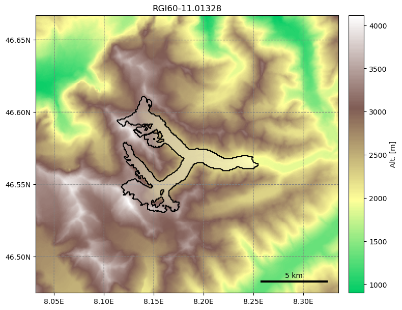
The advantage of this Glacier Directory data model is that it simplifies greatly the data transfer between tasks. The single mandatory argument of all entity tasks will allways be a glacier directory. With the glacier directory, each task will find the input it needs: for example, both the glacier’s topography and outlines are needed for the next plotting function, and both are available via the gdir argument:
from oggm import graphics
graphics.plot_domain(gdir, figsize=(8, 7))
Another advantage of glacier directories is their persistence on disk: once created, they can be recovered from the same location by using init_glacier_directories again, but without keyword arguments:
# Fetch the LOCAL pre-processed directories - note that no arguments are used!
gdirs = workflow.init_glacier_directories(rgi_ids)
2024-04-25 13:24:11: oggm.workflow: Execute entity tasks [GlacierDirectory] on 2 glaciers
See the store_and_compress_glacierdirs tutorial for more information on glacier directories.
Tasks#
There are two different types of “tasks”:
Entity Tasks: Standalone operations to be realized on one single glacier entity, independently from the others. The majority of OGGM tasks are entity tasks. They are parallelisable: the same task can run on several glaciers in parallel.
Global Task: Tasks which require to work on several glacier entities at the same time. Model parameter calibration or the compilation of several glaciers’ output are examples of global tasks.
OGGM implements a simple mechanism to run a specific task on a list of GlacierDirectory objects:
from oggm import tasks
# run the glacier_masks task on all gdirs
workflow.execute_entity_task(tasks.glacier_masks, gdirs);
2024-04-25 13:24:11: oggm.workflow: Execute entity tasks [glacier_masks] on 2 glaciers
The task we just applied to our list of glaciers is glacier_masks. It wrote a new file in our glacier directory, providing raster masks of the glacier (among other things):
print('Path to the masks:', gdir.get_filepath('gridded_data'))
Path to the masks: /tmp/OGGM/OGGM-GettingStarted/per_glacier/RGI60-11/RGI60-11.01/RGI60-11.01328/gridded_data.nc
It is also possible to apply several tasks sequentially (i.e. one after an other) on our glacier list:
list_talks = [
         tasks.compute_centerlines,
         tasks.initialize_flowlines,
         tasks.compute_downstream_line,
         ]
for task in list_talks:
    # The order matters!
    workflow.execute_entity_task(task, gdirs)
2024-04-25 13:24:12: oggm.workflow: Execute entity tasks [compute_centerlines] on 2 glaciers
2024-04-25 13:24:12: oggm.workflow: Execute entity tasks [initialize_flowlines] on 2 glaciers
2024-04-25 13:24:12: oggm.workflow: Execute entity tasks [compute_downstream_line] on 2 glaciers
The function execute_task can run a task on different glaciers at the same time, if the use_multiprocessing option is set to True in the configuration file.
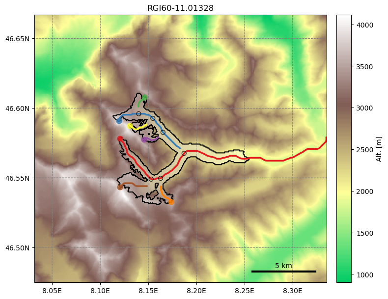
Among other things, we computed the glacier flowlines and the glacier’s downstream line. We can now plot them:
graphics.plot_centerlines(gdir, figsize=(8, 7), use_flowlines=True, add_downstream=True)
As a result, the glacier directories now store many more files. If you are interested, you can have a look:
import os
print(os.listdir(gdir.dir))
['model_flowlines.pkl', 'diagnostics.json', 'log.txt', 'flowline_catchments.tar.gz', 'catchments_intersects.tar.gz', 'inversion_output.pkl', 'inversion_input.pkl', 'dem.tif', 'outlines.tar.gz', 'inversion_flowlines.pkl', 'climate_historical.nc', 'downstream_line.pkl', 'mb_calib.json', 'geometries.pkl', 'glacier_grid.json', 'gridded_data.nc', 'centerlines.pkl', 'dem_source.txt', 'intersects.tar.gz']
For a short explanation of what these files are, see the glacier directory documentation. In practice, however, you will only rarely need to access these files yourself.
Other preprocessing tasks#
Let’s continue with the other preprocessing tasks:
list_talks = [
         tasks.catchment_area,
         tasks.catchment_width_geom,
         tasks.catchment_width_correction,
         tasks.compute_downstream_bedshape
         ]
for task in list_talks:
    # The order matters!
    workflow.execute_entity_task(task, gdirs)
2024-04-25 13:24:13: oggm.workflow: Execute entity tasks [catchment_area] on 2 glaciers
2024-04-25 13:24:15: oggm.workflow: Execute entity tasks [catchment_width_geom] on 2 glaciers
2024-04-25 13:24:16: oggm.workflow: Execute entity tasks [catchment_width_correction] on 2 glaciers
2024-04-25 13:24:16: oggm.workflow: Execute entity tasks [compute_downstream_bedshape] on 2 glaciers
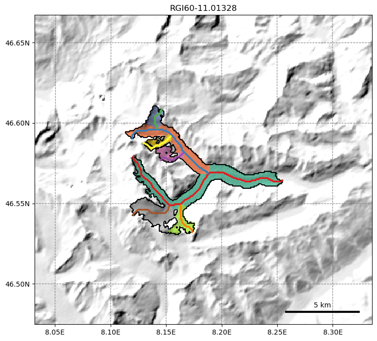
We just computed the catchment areas of each flowline (the colors are arbitrary):
graphics.plot_catchment_areas(gdir, figsize=(8, 7))
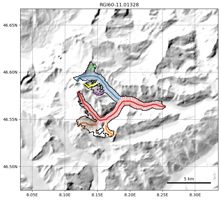
Each flowline now knows what area will contribute to its surface mass-balance and ice flow. Accordingly, it is possible to compute each glacier cross-section’s width, and correct it so that the total glacier area and elevation distribution is conserved:
graphics.plot_catchment_width(gdir, corrected=True, figsize=(8, 7))
Computing the ice thickness (“inversion”)#
With the computed mass-balance and the flowlines, OGGM can now compute the ice thickness, based on the principles of mass conservation and ice dynamics.
list_talks = [
         tasks.apparent_mb_from_any_mb,  # This is a preprocessing task
         tasks.prepare_for_inversion,  # This is a preprocessing task
         tasks.mass_conservation_inversion,  # This does the actual job
         tasks.filter_inversion_output  # This smoothes the thicknesses at the tongue a little
         ]
for task in list_talks:
    workflow.execute_entity_task(task, gdirs)
2024-04-25 13:24:19: oggm.workflow: Execute entity tasks [apparent_mb_from_any_mb] on 2 glaciers
2024-04-25 13:24:19: oggm.workflow: Execute entity tasks [prepare_for_inversion] on 2 glaciers
2024-04-25 13:24:19: oggm.workflow: Execute entity tasks [mass_conservation_inversion] on 2 glaciers
2024-04-25 13:24:19: oggm.workflow: Execute entity tasks [filter_inversion_output] on 2 glaciers
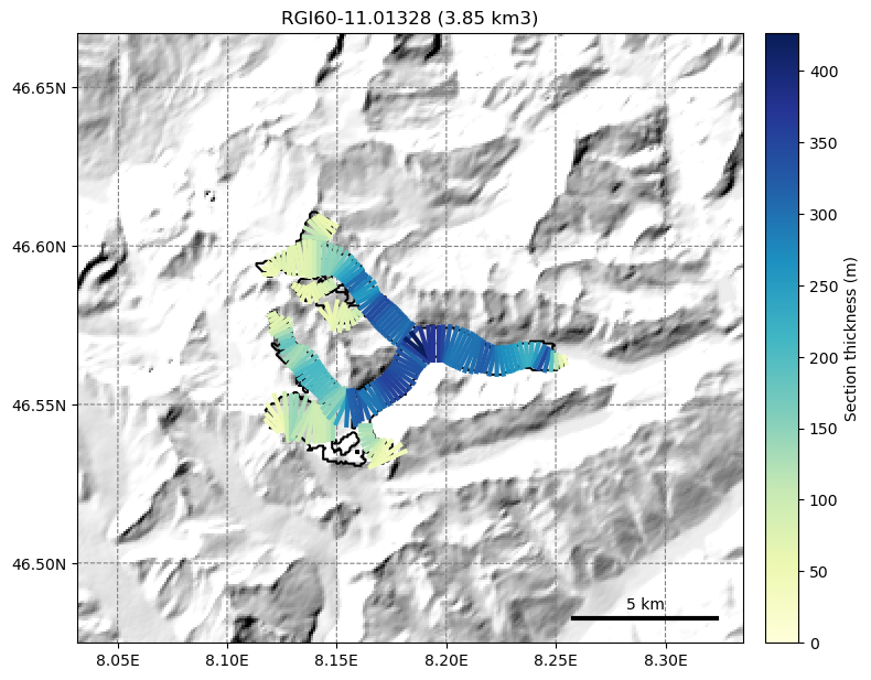
The ice thickness is computed for all sections along the flowline, and can be displayed with the help of OGGM’s graphics module:
graphics.plot_inversion(gdir, figsize=(8, 7))
The inversion is realized with the default parameter settings: it must be noted that the model is sensitive to the choice of some of them, most notably the creep parameter A:
cfg.PARAMS['inversion_glen_a']
2.4e-24
import numpy as np
import matplotlib.pyplot as plt

a_factor = np.linspace(0.1, 10., 100)
volume = []
for f in a_factor:
    # Recompute the volume without overwriting the previous computations
    v = tasks.mass_conservation_inversion(gdir, glen_a=f * cfg.PARAMS['inversion_glen_a'], write=False)
    volume.append(v * 1e-9)
plt.plot(a_factor, volume); plt.title('Unteraar total volume');
plt.ylabel('Volume (km$^3$)'); plt.xlabel('Glen A factor (1 = default)');
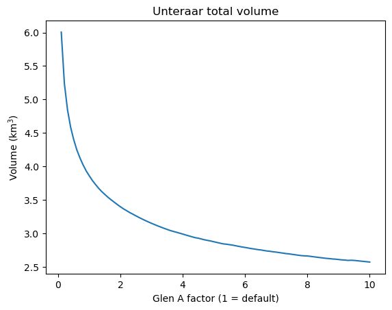
There is no simple way to find the best A for each individual glacier. It can easily vary by a factor of 10 (or more) from one glacier to another. At the global scale, the “best” A is close to the default value (possibly between 1 and 1.5 times larger). The default parameter a good choice in a first step but be aware that reconstructions based on this default parameter might be very uncertain! See our ice thickness inversion tutorial for a more in-depth discussion.
Simulations#
For most applications, this is where the fun starts! With climate data and an estimate of the ice thickness, we can now start transient simulations. For this tutorial, we will show how to realize idealized experiments based on the baseline climate only, but it is also possible to drive OGGM with real GCM data.
# Convert the flowlines to a "glacier" for the ice dynamics module
workflow.execute_entity_task(tasks.init_present_time_glacier, gdirs);
2024-04-25 13:24:21: oggm.workflow: Execute entity tasks [init_present_time_glacier] on 2 glaciers
Let’s start a run driven by a the climate of the last 31 years, shuffled randomly for 200 years. This can be seen as a “commitment” simulation, i.e. how much glaciers will change even without further climate change:
cfg.PARAMS['store_model_geometry'] = True  # add additional outputs for the maps below
cfg.PARAMS['evolution_model'] = 'FluxBased'
workflow.execute_entity_task(tasks.run_random_climate, gdirs, nyears=200,
                             y0=2000, output_filesuffix='_2000');
2024-04-25 13:24:21: oggm.cfg: PARAMS['store_model_geometry'] changed from `False` to `True`.
2024-04-25 13:24:21: oggm.cfg: PARAMS['evolution_model'] changed from `SemiImplicit` to `FluxBased`.
2024-04-25 13:24:21: oggm.workflow: Execute entity tasks [run_random_climate] on 2 glaciers
The output of this simulation is stored in two separate files: a diagnostic file (which contains time series variables such as length, volume, ELA, etc.) and a full model output file, which is larger but allows to reproduce the full glacier geometry changes during the run.
In practice, the diagnostic files are often compiled for the entire list of glaciers:
ds2000 = utils.compile_run_output(gdirs, input_filesuffix='_2000')
2024-04-25 13:24:43: oggm.utils: Applying global task compile_run_output on 2 glaciers
2024-04-25 13:24:43: oggm.utils: Applying compile_run_output on 2 gdirs.
This dataset is also stored on disk (in the working directory) as NetCDF file for later use. Here we can access it directly:
ds2000
<xarray.Dataset> Size: 31kB
Dimensions:         (time: 201, rgi_id: 2)
Coordinates:
  * time            (time) float64 2kB 0.0 1.0 2.0 3.0 ... 198.0 199.0 200.0
  * rgi_id          (rgi_id) <U14 112B 'RGI60-11.01328' 'RGI60-11.00897'
    hydro_year      (time) int64 2kB 0 1 2 3 4 5 6 ... 195 196 197 198 199 200
    hydro_month     (time) int64 2kB 4 4 4 4 4 4 4 4 4 4 ... 4 4 4 4 4 4 4 4 4 4
    calendar_year   (time) int64 2kB 0 1 2 3 4 5 6 ... 195 196 197 198 199 200
    calendar_month  (time) int64 2kB 1 1 1 1 1 1 1 1 1 1 ... 1 1 1 1 1 1 1 1 1 1
Data variables:
    volume          (time, rgi_id) float64 3kB 3.849e+09 8.617e+08 ... 2.745e+08
    volume_bsl      (time, rgi_id) float64 3kB 0.0 0.0 0.0 0.0 ... 0.0 0.0 0.0
    volume_bwl      (time, rgi_id) float64 3kB 0.0 0.0 0.0 0.0 ... 0.0 0.0 0.0
    area            (time, rgi_id) float64 3kB 2.383e+07 8.036e+06 ... 4.845e+06
    length          (time, rgi_id) float64 3kB 1.342e+04 6.9e+03 ... 1.9e+03
    calving         (time, rgi_id) float64 3kB 0.0 0.0 0.0 0.0 ... 0.0 0.0 0.0
    calving_rate    (time, rgi_id) float64 3kB 0.0 0.0 0.0 0.0 ... 0.0 0.0 0.0
    water_level     (rgi_id) float64 16B 0.0 0.0
    glen_a          (rgi_id) float64 16B 2.4e-24 2.4e-24
    fs              (rgi_id) float64 16B 0.0 0.0
Attributes:
    description:    OGGM model output
    oggm_version:   1.6.2.dev35+g7489be1
    calendar:       365-day no leap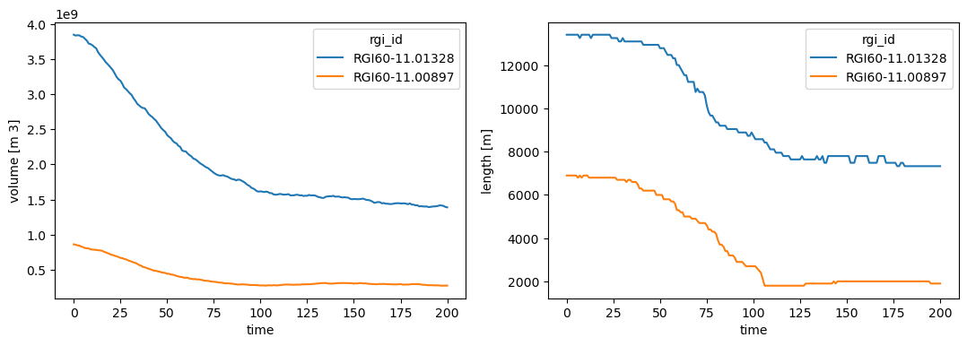
creation_date: 2024-04-25 13:24:43We opened the file with xarray, a very useful data analysis library based on pandas. For example, we can plot the volume and length evolution of both glaciers with time:
f, (ax1, ax2) = plt.subplots(1, 2, figsize=(13, 4))
ds2000.volume.plot.line(ax=ax1, hue='rgi_id');
ds2000.length.plot.line(ax=ax2, hue='rgi_id');
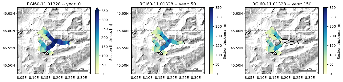
The full model output files can be used for plots:
f, (ax1, ax2, ax3) = plt.subplots(1, 3, figsize=(14, 6))
graphics.plot_modeloutput_map(gdir, filesuffix='_2000', modelyr=0, ax=ax1, vmax=350)
graphics.plot_modeloutput_map(gdir, filesuffix='_2000', modelyr=50, ax=ax2, vmax=350)
graphics.plot_modeloutput_map(gdir, filesuffix='_2000', modelyr=150, ax=ax3, vmax=350)
plt.tight_layout();
Sensitivity to temperature#
Now repeat our simulations with a +0.5°C and -0.5°C temperature bias, which for a glacier is quite a lot!
workflow.execute_entity_task(tasks.run_random_climate, gdirs, nyears=200,
                             temperature_bias=0.5,
                             y0=2000, output_filesuffix='_p05');
workflow.execute_entity_task(tasks.run_random_climate, gdirs, nyears=200,
                             temperature_bias=-0.5,
                             y0=2000, output_filesuffix='_m05');
2024-04-25 13:24:51: oggm.workflow: Execute entity tasks [run_random_climate] on 2 glaciers
2024-04-25 13:25:11: oggm.workflow: Execute entity tasks [run_random_climate] on 2 glaciers
dsp = utils.compile_run_output(gdirs, input_filesuffix='_p05')
dsm = utils.compile_run_output(gdirs, input_filesuffix='_m05')
2024-04-25 13:25:33: oggm.utils: Applying global task compile_run_output on 2 glaciers
2024-04-25 13:25:33: oggm.utils: Applying compile_run_output on 2 gdirs.
2024-04-25 13:25:33: oggm.utils: Applying global task compile_run_output on 2 glaciers
2024-04-25 13:25:33: oggm.utils: Applying compile_run_output on 2 gdirs.
f, (ax1, ax2, ax3) = plt.subplots(1, 3, figsize=(16, 4))
rgi_id = 'RGI60-11.01328'
ds2000.sel(rgi_id=rgi_id).volume.plot.line(ax=ax1, hue='rgi_id', label='Commitment');
ds2000.sel(rgi_id=rgi_id).area.plot.line(ax=ax2, hue='rgi_id');
ds2000.sel(rgi_id=rgi_id).length.plot.line(ax=ax3, hue='rgi_id');
dsp.sel(rgi_id=rgi_id).volume.plot.line(ax=ax1, hue='rgi_id', label='$+$ 0.5°C');
dsp.sel(rgi_id=rgi_id).area.plot.line(ax=ax2, hue='rgi_id');
dsp.sel(rgi_id=rgi_id).length.plot.line(ax=ax3, hue='rgi_id');
dsm.sel(rgi_id=rgi_id).volume.plot.line(ax=ax1, hue='rgi_id', label='$-$ 0.5°C');
dsm.sel(rgi_id=rgi_id).area.plot.line(ax=ax2, hue='rgi_id');
dsm.sel(rgi_id=rgi_id).length.plot.line(ax=ax3, hue='rgi_id');
ax1.legend();
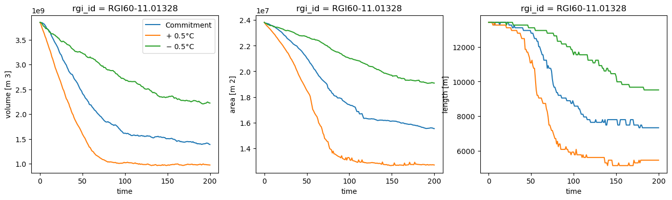
From this experiment, we learn that a climate that is -0.5° colder than today (i.e. mean climate of 1985-2015) would barely be enough to maintain the Unteraar glacier in its present day geometry.
What’s next?#
return to the OGGM documentation
back to the table of contents