During last week’s glaciological field course Stephan and I tried to explain the pros and cons of using the specific mass-balance as standard monitoring variable for the long-term mass-balance timeseries.
As a reminder, the term specific mass-balance (SMB) refers to a mass-balance per unit area, preferably1 averaged over the entire glacier (with units2 of [kg m$^{-2}$]). The SMB is measurable using conventional mass-balance measurements methods and has been the standard since glacier measurements exist.
The problem with the specific mass-balance is that it is not only dependent on the climate but also on the changing glacier surface. The debate about whether SMB is appropriate for climate-crysophere interactions studies is not new (see e.g. this online comment from 2010 and the associated author response), and this blog post is not an attempt to settle this debate.
The purpose of this post is rather to demonstrate that OGGM can (also) be used for educational purposes: here, to illustrate the non-linear response of SMB to changes in climate.
Set-up
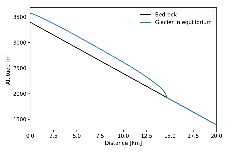
We start with an idealised glacier in equilibrium with a constant climate. We use a linear mass-balance gradient with an Equilibrium Line Altitude (ELA) is set to 2900 m a.s.l. At equilibrium, exactly half of the glacier is located in the accumulation and ablation zone3. With a parabolic bed shape we obtain a glacier of length 15 km and area 6 km$^{2}$, corresponding to a medium to large sized glacier for the Alps (for example the Hintereisferner in the Austrian Alps).
We look at the evolution of this glacier under two scenarios: a response to a brutal step-wise change of climate and to a slow, regular climate trend.
Step-wise change in climate
After 50 years at a constant climate, the ELA is increased of 150 m (roughly corresponding to a change in temperature of 1 K). The figure below shows the glacier response over time (area and SMB):
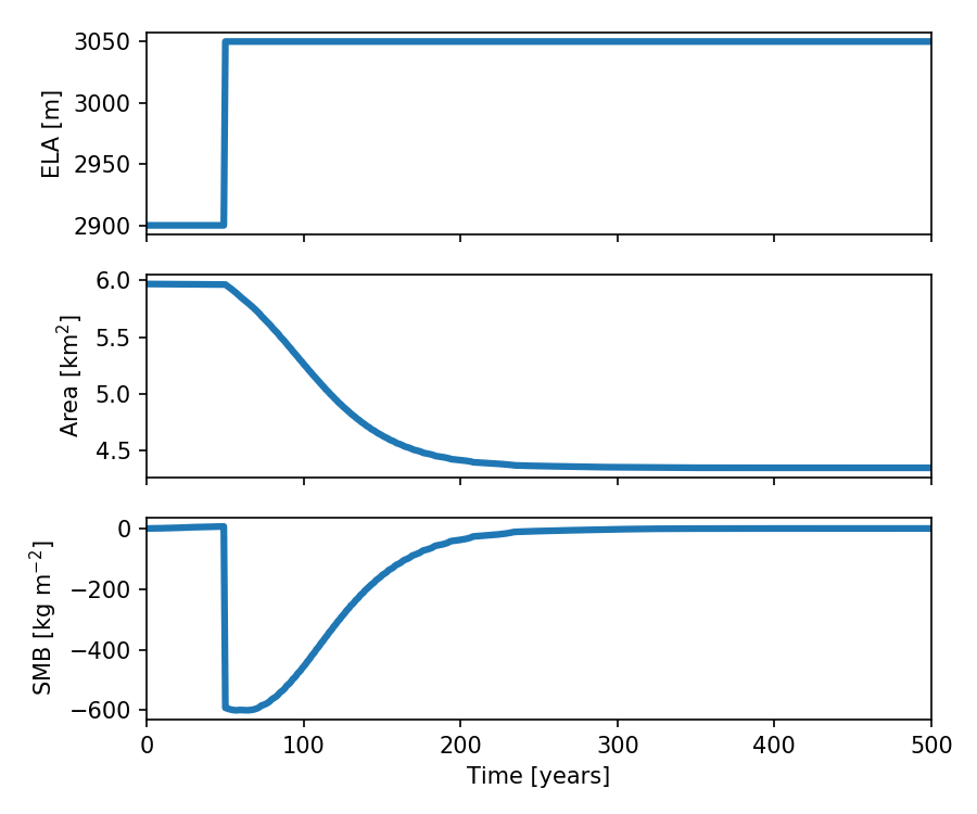
After the abrupt climate change, the accumulation area is reduced and the ablation is stronger: the glacier shrinks and reaches a new equilibrium state after about 200 years. Before the change the SMB is zero (as expected from a glacier in equilibrium), but after the shift the SMB displays a discontinuous step followed by a logarithmic recovery to equilibrium. Indeed, the smaller the glacier, the smaller its imbalance with climate.
The interesting bit about this experiment is that if an observer starts a mass-balance monitoring program at year 51, she will notice a positive trend in SMB! This could be easily misinterpreted as a (non-existent) cooling in climate.
A more “realistic” scenario
This time, we let the ELA rise linearly between the same two levels as in the previous experiment. The “climate change” now happens over a 300 years period (i.e. slower than the current anthropogenic climate change):
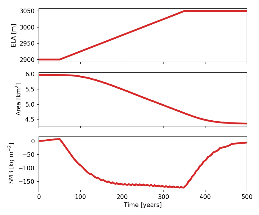
With this scenario, the glacier reaches the same equilibrium area as with a step-wise climate change, but after a longer time of course. After the end of the climate trend, the equilibrium is reached in about 150 years.
Did you expect such a behavior in the SMB? A striking feature is that the SMB signal is strongly non linear: after a certain time the elevation feedback3 kicks in and the SMB reaches a more or less constant value. From year 200 to 350 the glacier responds “equally” to past and present climate change and has no “memory” from its previous equilibrium state.
Here again, a glaciologist would have a hard time to reconstruct a climate signal from the observed SMB curve.
In reality, however, glaciers are more likely to respond faster to climate change. The SMB of smaller glaciers, in particular, is a very good indicator of climate variability. These experiments demonstrate however that the SMB of larger glaciers needs to be interpreted with caution.
What about the ELA?
This is why some glaciologist prefer to use the ELA as indicator for climate change. Especially at very long (paleo) time scales, the ELA is much preferred to other mass-balance indicators. The problem with ELA however is that is doesn’t take into account that the mass-balance gradients might also change in time…
To go further
There are plenty of other experiments we could do with this simple set-up. For example:
- how does the SMB evolution changes with varying trend intensities in ELA?
- what happens in a more realistic climate, i.e. when natural variability is superposed to the trend?
- what happens in the case of a smaller glacier? a larger one?
- …
These questions are left open for the reader ;)
Notes
The code used to generate these plots can be found in the OGGM repository.
-
refer to the Glossary of glacier mass balance and related terms for a widely accepted definition. ↩
-
[kg m$^{-2}$] is equivalent to the frequently used [mm w.e. m$^{-2}$]. The latter is not S.I. compliant though. ↩
-
the elevation feedback refers to the fact that a thiner glacier will have a more negative mass-balance than a thicker one, simply because its elevation is lower. ↩ ↩2