A very typical situation in geosciences is that a numerical model (here called “impact model”) is driven by forcing data (often: reanalysis data or climate model output). There are many impact models around: hydrological models and glacier models are obvious ones.
Take home message
This blog post has one simple message to convey (not new, but written here again for reference):
Do not average the forcing data before giving it to an impact model that has been trained on a different temporal resolution.
Let $M$ be the non-linear impact model, and $X$ the forcing data variables (temperature, precipitation, etc.). Therefore, $M(X)$ is the output of the impact model.
Now let $\overline{X}$ be the average of the variable $X$ (either a temporal average, a climatology over 30 years, or the average of several ensemble members). Accordingly, $\overline{M(X)}$ is the average of the model output after being forced by $X$ (not averaged). $\overline{M(X)}$ is the true average value of the quantity we are interested in.
Then, it is easy to show that if $M$ is a non-linear impact model (like most models), the following model results are not equivalent:
$\overline{M(X)} \neq M(\overline{X})$
The example of the degree day model
In the very famous degree day melt model, the daily melt $m$ is computed as:
$ M = \mu T \text{ if } T\geq 0 \text{, and } M = 0 \text{ otherwise}$
with $\mu$ a calibrated melt factor (let’s assume it is $\mu = 1$ here).
Then, lets say we want to compute the melt on Oct. 1 of five consecutive years. For four years, the temperature was -2°C, then on the fifth it was 5°C. Then, $\overline{M(X)} = 5 / 5 = 1$. However, $M(\overline{X}) = M(0 / 5) = 0$.
Note 1: a “degree day model” is already an averaging and a simplification: what is not correct here is the further averaging.
Note 2: from the example above, it may seem that monthly degree days models are not possible: see below for for a discussion.
What to do about it?
There are a few situations where you may still want or need to average your inputs before feeding them to a model. Here are a few common situations with suggested solutions:
Monthly “degree day” models
A model at monthly resolution is often needed because the forcing data (e.g. GCM data) may not be available at a higher resolution. To avoid confusion, we prefer to call them “temperature index models” in the OGGM documentation. Here are some known available strategies to deal with monthly data:
- you can calibrate a model using monthly resolution data. It may imply to recalibrate the temperature melt threshold to value below 0°C to take into account months with negative average temperatures might have positive melt days. This is the solution chosen by Marzeion et al., (2012) and OGGM (v1).
- you can use monthly averages and an estimate of variability to reconstruct daily temperatures, either with random numbers (Huss & Hock, 2015; Rounce et al., 2020) or a more deterministic but computationally expensive quantile based method (OGGM sandbox).
Constant average climate forcing
This is a further typical use case: say you want to compute the “committed glacier mass loss”, i.e. the mass that would be lost if the climate of the last decades would “stabilize”.
The first forcing method is to repeat the timeseries of the last decades in a loop, until the glaciers have stabilized. This is the simplest method and the one used by Marzeion et al., (2018).
The second forcing method is very similar, but consists of shuffling the years randomly instead of repeating the timeseries in a loop. This avoids unwanted effects related to a cyclic forcing.
The third forcing method consists of feeding the glacier geometry evolution model with an average of the periods mass-balance, by computing $\overline{M(X)}$:
- for a given glacier glacier geometry at year
y0, compute the mass-balance over the climate period you are interested in. - average the output over time (i.e. compute $\overline{M(X)}$) and give this value to the glacier geometry evolution model.
- compute the new glacier geometry at
y1and repeat from (1).
As you see, this third method implies to compute N years of mass-balance (often: 20 or 30) each year of glacier evolution, because of the geometry update. This is quite computationally expensive. Therefore, the standard procedure in OGGM (the ConstantMassBalance model class) is to compute the N years signal only once for a wide range of elevation bins, and then interpolate between them after each geometry update, which is faster.
A fourth method might consist of recalibrating the model using an average climate instead (like we did when using monthly degree day models). This method still ignores one important aspect of climate: its variability.
For more information on this use case, visit our next blog post which goes into more detail.
Model ensemble
Another very often encounter is an ensemble of forcing data simulations (e.g. CMIP). For this use case, there is no simple solution (at least with temperature index models) and the only reasonable way is to force your model realisation and then average the signal.
If you want more information about why we write this down today, here is what Anouk Vlug found out the hard way during her PhD thesis:
I have been amazed by the impact that climate variability had in my glacier simulations, to the extent that I wondered “what can go so wrong?” Here is an illustration:
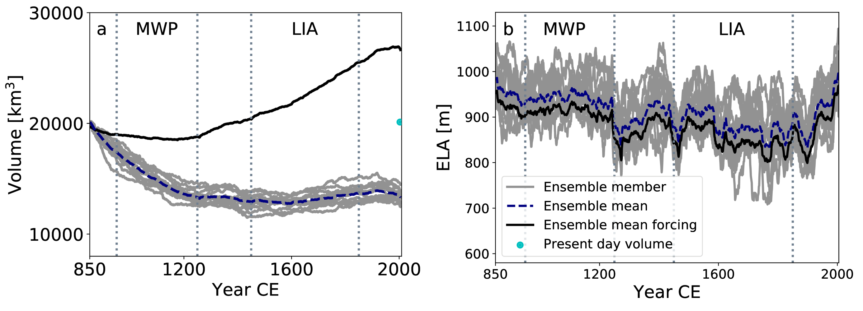
The experiment includes most of the land-terminating glaciers in the Canadian Arctic. For the glacier simulations, OGGM was forced with the 13 fully forced ensemble members from the Community Earth System Model Last Millennium Ensemble (CESM-LME) individually at first, and then with the ensemble mean. In the figure you can see that this leads to a very different evolution of the glacier volume in the region. The simulation that was forced with the ensemble mean is very different from the mean of the ensemble, and lies far outside the spread of the simulations that were forced with the individual ensemble members.
So, why does this happen? It is because of the effect of the averaging illustrated above. When the ensemble members are averaged, this strongly reduces the temperature variability. So much, in fact, that much fewer years in the averaged timeseries lead to glacier melt, and therefore the glaciers are now growing instead of shrinking!