Following ongoing discussions with colleagues about the GlacierMIP3 experiment, I thought that it would be good to further explain the methods listed in a previous blog post, using concrete examples with OGGM.
The objective of the GlacierMIP3 simulations are to simulate glacier evolution under various “stable climates”. For example, how would glaciers change if the climate of 2000-2021 (21 years) remained stable? A “stable climate” is a purely theoretical scenario, since in reality climate always changes. It is highly unlikely that statistical measures such as the average and standard deviation of temperature do not change with time. However, we expect these simulations to be of high scientific and policy-relevant value, since they will show “what if?” scenarios outcomes in a controlled global experiment.
The objective of this blog post is to explain how OGGM computes glacier mass-balance, and why the design of these theoretical experiments matters to us. Although these examples are OGGM specific, I believe that some of these results are applicable to other models as well.
A few definitions
In OGGM, we have a clear separation between the glacier geometry evolution model and the glacier mass-balance model.
The geometry evolution model needs to know the mass-balance of the glacier at regular time intervals and varying elevations along the glacier. The default is to do a yearly update: in practice, this means that the geometry evolution model knows the altitude area distribution of the glacier at year y0, asks the mass-balance model to provide the y0 annual mass-balance at each grid point along the geometry, and then computes the geometry evolution accordingly. At y1, with the new geometry, the mass-balance model is asked again to provide the new mass-balance for y1, etc.
The fact that the geometry evolution model needs climate at annual time steps has no influence whatsoever on the time resolution of the mass-balance model. The mass-balance model can for example compute the mass-balance at hourly or annual time steps, as long as it provides the annual mass-balance to the geometry evolution model. In OGGM, the current default is to compute mass-balance at monthly time steps: for any given year, the monthly data is used to compute the 12 months of mass-balance, summed and provided to the geometry evolution model. The model used here is a monthly temperature index model as described in Marzeion et al., (2012) and Maussion et al., (2019).
Forcing methods
I am going to illustrate three different forcing methods implemented in OGGM, all three meant to represent the theoretical equilibrium experiment that we wish to realize in GlacierMIP3.
Method 1 (AvgClim) uses multi-year monthly averages of the climate data to force the mass-balance model. In practice, we compute a monthly climatology of the temperature and precipitation time series. We then use the OGGM monthly mass-balance model to compute the mass-balance based on this monthly climatology. The mass-balance profile provided to the geometry evolution model is the same each year (it is only a function of elevation, not of time).
Method 2 (AvgMB) drives the mass-balance model with monthly data of the entire entire simulation period (for example, 2000-2020), hence the monthly climate data varies from year to year. We then calculate average monthly mass-balance profiles over all years of the simulation period, which is then converted into a mean annual mass-balance profile. The geometry evolution model is then forced repeatedly with this mean annual mass-balance profile. Like for Method 1, the mass-balance profile provided to the geometry evolution model is the same each year (it is only a function of elevation, not of time).
Method 3 (RdnMB) uses a random number generator to create a synthetic time series of climate. Each given year is picked randomly from the (2000-2020) period. In this process, we are careful not to pick the same year twice within a 21 year period. Unlike Method 1 and 2, the annual mass-balance provided to the geometry evolution model at a given elevation changes each year.
Example 1: Hintereisferner, reference period 2000-2020
Here is a plot showing the monthly specific mass-balance computed by the mass-balance model over a fixed glacier geometry using the three methods above:
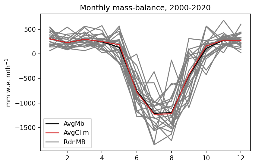
The random climate randomly shifts between the grey lines, while the two other methods compute a time invariant mass-balance. The differences between Method 1 and Method 2 are small, but most visible in the transition periods, in the months where the temperature varies above and below the melting temperature threshold (more on this below).
The annual specific mass-balance averages are -1684, -1739, and -1739 mm w.e. yr$^{-1}$ for each of the three methods, respectively. Method 2 and 3 have the same average, per construction. The reason why Method 1 differs is explained in the previous blog post: it is due to the presence of non-linear equations in the mass-balance model.
Now, let’s see what happens if we run the full model (glacier mass-balance + glacier evolution) for a period of 300 years using this three forcing scenarios:
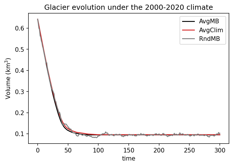
So far so good! In the strongly retreating case, all forcing methods lead to similar results. Now let’s see what happens in a colder scenario.
Example 2: Hintereisferner, reference period 1960-1980
In the 60s and 70s, Hintereisferner was close to balance and even had several positive years, leading to a positive average mass-balance over that period (with the present day glacier geometry).
Now let’s have a look at the plots again with this time period:
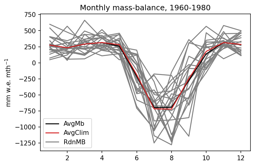
The annual specific mass-balance averages are 303, 241, and 241 mm w.e. yr$^{-1}$, respectively. For the volume evolution, these relative differences have larger consequences:
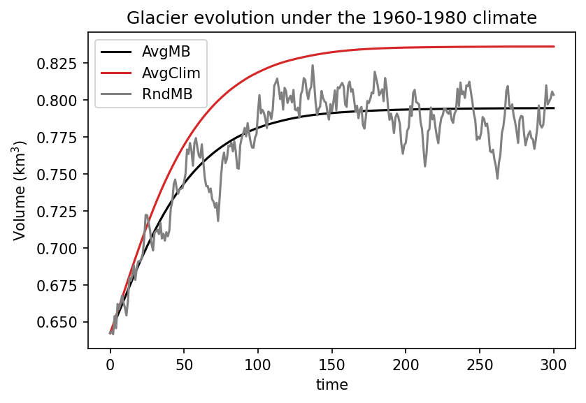
That’s quite a difference now. Why does this happen? In OGGM at least, the melting temperature threshold (the monthly temperature at which melt occurs) is a global parameter (set at -1°C per default). The more months we have where the temperature is oscillating around this threshold, the more likely it is that the average climate is actually below this threshold. This leads to non-linear effects, which are small in the grand scheme of things but become increasingly relevant in the equilibrium scenarios, where glaciers are slowly adapting to a theoretical, stable climate. In these theoretical scenarios, even a few mm w.e. matter a lot! Indeed, when a glacier grows a positive feedback occurs: the mass-balance / elevation feedback, which tends to amplify the original signal.
Conclusions
In OGGM at least, Methods 2 and 3 are viable options to represent the climate of a given period (although we agree that this is a theoretical experiment). Method 1, although being easy to apply, lead to different mass-balance estimates. This is even more relevant when considering model calibration to geodetic estimates, where only Methods 2 and 3 will guarantee consistency between the calibration and the application of the mass-balance model.
It must be noted that more advanced models using internal representations of daily variability might be less sensitive than OGGM to such choices. Using daily emulators is standard practice in GloGEM and PyGEM, but not yet in OGGM. The new generation of mass-balance models (massbalance-sandbox developed by Lilian Schuster) now offer such models to our users. Our first experiments with this model shows very similar responses and sensitivity to the choice of the forcing method, with method 2 and 3 leading to similar results and method 1 showing a systematic difference. The sign of this difference (if positive or negative) is not systematic and may change from glacier to glacier or with climate conditions.
Code & Data
The code used to create these plots is available here.