Selecting glaciers in a shapefile, selecting data, running OGGM for a list of glaciers

In this notebook we will:

• show how to select glaciers in a basin using a shapefile

• show how to use published runoff data for this basin

• use OGGM on a list of glaciers

import geopandas as gpd

import xarray as xr
import salem
import numpy as np
import pandas as pd

import matplotlib.pyplot as plt
import seaborn as sns
sns.set_context('notebook') 

import oggm.cfg
from oggm import utils, workflow, tasks, graphics

# OGGM options
oggm.cfg.initialize(logging_level='WARNING')

2023-03-23 08:48:58: oggm.cfg: Reading default parameters from the OGGM `params.cfg` configuration file.

2023-03-23 08:48:58: oggm.cfg: Multiprocessing switched OFF according to the parameter file.

2023-03-23 08:48:58: oggm.cfg: Multiprocessing: using all available processors (N=8)

Reading the RGI file

RGI can be downloaded freely. In OGGM we offer to read them for you:

from oggm import utils
rgi_file = utils.get_rgi_region_file(14, version='62')  # This is East Asia

# Read it
rgi_df = gpd.read_file(rgi_file)

f"The region has {len(rgi_df)} glaciers and an area of {rgi_df['Area'].sum()}km2"

'The region has 27988 glaciers and an area of 33568.298km2'

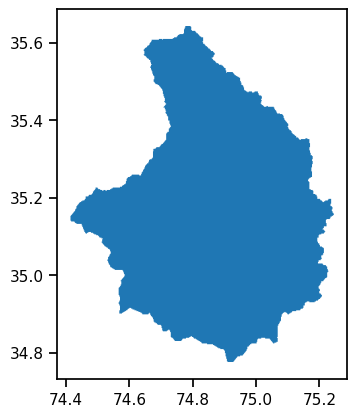
Selecting glaciers in a basin

This file can be downloaded here and added to the folder of the notebook.

fpath = 'zip://Astore.zip/Astore'
basin_df = gpd.read_file(fpath)

basin_df.plot();

We can select all glaciers within this shape by using their center point:

import shapely.geometry as shpg
in_basin = [basin_df.geometry.contains(shpg.Point(x, y))[0] for (x, y) in zip(rgi_df.CenLon, rgi_df.CenLat)]
rgi_df_sel = rgi_df.loc[in_basin]

ax = basin_df.plot();
rgi_df_sel.plot(ax=ax, edgecolor='k');

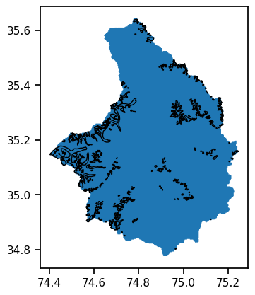
f"The Astore region has {len(rgi_df_sel)} glaciers and an area of {rgi_df_sel['Area'].sum():.2f} km2"

'The Astore region has 357 glaciers and an area of 256.53 km2'

Optional: fancy plot

# One interactive plot below requires Bokeh
# The rest of the notebook works without this dependency - comment if needed
import holoviews as hv
hv.extension('bokeh')
import geoviews as gv
import geoviews.tile_sources as gts

(gv.Polygons(rgi_df_sel[['geometry']]).opts(fill_color=None, color_index=None) * gts.tile_sources['EsriImagery'] * 
 gts.tile_sources['StamenLabels']).opts(width=750, height=500, active_tools=['pan', 'wheel_zoom'])

Read the Rounce et al. (2023) projections and select the data

These data are provided by Rounce et al., 2023 (download). The whole global dataset is available here: https://nsidc.org/data/hma2_ggp/versions/1

We prepared data for the entire Indus basin for you. You can download them in different selections here: https://cluster.klima.uni-bremen.de/~fmaussion/share/world_basins/rounce_data

Here we illustrate how to select data for Astore out of the much larger Indus file, which contains more than 25k glaciers!

import xarray as xr

# Take the data as numpy array
rgi_ids = rgi_df_sel['RGIId'].values

# This path works on classroom.oggm.org! To do the same locally download the data and open it from there
# path = '/home/www/fmaussion/share/world_basins/rounce_data/Indus/runoff_rounce_INDUS_ssp126_monthly.nc'
# If you work elsewhere, you can use this:
path = utils.file_downloader('https://cluster.klima.uni-bremen.de/~fmaussion/share/world_basins/rounce_data/Indus/runoff_rounce_INDUS_ssp126_monthly.nc')

# This might take a minute, as it extracts data from a large file
# Sometimes a random HDF error occurs on classroom - I'm not sure why...
with xr.open_dataset(path) as ds:
    # This selects the 357 glaciers out of many thousands
    ds_rounce_ssp126 = ds.sel(rgi_id=rgi_ids).load()

Let’s have a look at the data now:

ds_rounce_ssp126

<xarray.Dataset>
Dimensions:                    (time: 1212, rgi_id: 357, gcm: 12)
Coordinates:
  * time                       (time) datetime64[ns] 2000-01-01 ... 2100-12-01
  * rgi_id                     (rgi_id) object 'RGI60-14.19043' ... 'RGI60-14...
  * gcm                        (gcm) object 'BCC-CSM2-MR' ... 'NorESM2-MM'
    ssp                        <U6 'ssp126'
Data variables: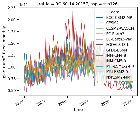
    glac_runoff_fixed_monthly  (gcm, rgi_id, time) float64 0.0 0.0 ... 0.0 0.0

xarray.Dataset

• Dimensions:
  • time: 1212
  • rgi_id: 357
  • gcm: 12
• Coordinates: (4)
  • time
    (time)
    datetime64[ns]
    2000-01-01 ... 2100-12-01

    long_name :

    time

    range :

    2000 - 2101

    comment :

    start of the month

    array(['2000-01-01T00:00:00.000000000', '2000-02-01T00:00:00.000000000',
           '2000-03-01T00:00:00.000000000', ..., '2100-10-01T00:00:00.000000000',
           '2100-11-01T00:00:00.000000000', '2100-12-01T00:00:00.000000000'],
          dtype='datetime64[ns]')

  • rgi_id
    (rgi_id)
    object
    'RGI60-14.19043' ... 'RGI60-14.2...

    array(['RGI60-14.19043', 'RGI60-14.19044', 'RGI60-14.19045', ...,
           'RGI60-14.20241', 'RGI60-14.20252', 'RGI60-14.20254'], dtype=object)

  • gcm
    (gcm)
    object
    'BCC-CSM2-MR' ... 'NorESM2-MM'

    array(['BCC-CSM2-MR', 'CESM2', 'CESM2-WACCM', 'EC-Earth3', 'EC-Earth3-Veg',
           'FGOALS-f3-L', 'GFDL-ESM4', 'INM-CM4-8', 'INM-CM5-0', 'MPI-ESM1-2-HR',
           'MRI-ESM2-0', 'NorESM2-MM'], dtype=object)

  • ssp
    ()
    <U6
    'ssp126'

    array('ssp126', dtype='<U6')

• Data variables: (1)
  • glac_runoff_fixed_monthly
    (gcm, rgi_id, time)
    float64
    0.0 0.0 0.0 0.0 ... 0.0 0.0 0.0

    description: :

    monthly glacier runoff for almost all glaciers of the Indus basin (two are missing). Runoff is calculated assuming a fixed gauge (i.e., it includes on-glacier and off-glacier runoff as glacier starts to retreat and represents runoff from a fixed gauge at a glacier terminus that does not move over time).

    unit: :

    kg month-1

    data source: :

    Rounce, D.R., R. Hock, and F. Maussion. 2022. Global PyGEM-OGGM Glacier Projections with RCP and SSP Scenarios, Version 1. [glac_runoff_fixed_monthly, RGI region 13 & 14] Boulder, Colorado USA. NASA National Snow and Ice Data Center Distributed Active Archive Center. https://doi.org/10.5067/P8BN9VO9N5C7. [10-01-2023]. Aggregated by Lilian Schuster.

    array([[[0., 0., 0., ..., 0., 0., 0.],
            [0., 0., 0., ..., 0., 0., 0.],
            [0., 0., 0., ..., 0., 0., 0.],
            ...,
            [0., 0., 0., ..., 0., 0., 0.],
            [0., 0., 0., ..., 0., 0., 0.],
            [0., 0., 0., ..., 0., 0., 0.]],
    
           [[0., 0., 0., ..., 0., 0., 0.],
            [0., 0., 0., ..., 0., 0., 0.],
            [0., 0., 0., ..., 0., 0., 0.],
            ...,
            [0., 0., 0., ..., 0., 0., 0.],
            [0., 0., 0., ..., 0., 0., 0.],
            [0., 0., 0., ..., 0., 0., 0.]],
    
           [[0., 0., 0., ..., 0., 0., 0.],
            [0., 0., 0., ..., 0., 0., 0.],
            [0., 0., 0., ..., 0., 0., 0.],
            ...,
    ...
            ...,
            [0., 0., 0., ..., 0., 0., 0.],
            [0., 0., 0., ..., 0., 0., 0.],
            [0., 0., 0., ..., 0., 0., 0.]],
    
           [[0., 0., 0., ..., 0., 0., 0.],
            [0., 0., 0., ..., 0., 0., 0.],
            [0., 0., 0., ..., 0., 0., 0.],
            ...,
            [0., 0., 0., ..., 0., 0., 0.],
            [0., 0., 0., ..., 0., 0., 0.],
            [0., 0., 0., ..., 0., 0., 0.]],
    
           [[0., 0., 0., ..., 0., 0., 0.],
            [0., 0., 0., ..., 0., 0., 0.],
            [0., 0., 0., ..., 0., 0., 0.],
            ...,
            [0., 0., 0., ..., 0., 0., 0.],
            [0., 0., 0., ..., 0., 0., 0.],
            [0., 0., 0., ..., 0., 0., 0.]]])

• Indexes: (3)
  • time
    PandasIndex

    PandasIndex(DatetimeIndex(['2000-01-01', '2000-02-01', '2000-03-01', '2000-04-01',
                   '2000-05-01', '2000-06-01', '2000-07-01', '2000-08-01',
                   '2000-09-01', '2000-10-01',
                   ...
                   '2100-03-01', '2100-04-01', '2100-05-01', '2100-06-01',
                   '2100-07-01', '2100-08-01', '2100-09-01', '2100-10-01',
                   '2100-11-01', '2100-12-01'],
                  dtype='datetime64[ns]', name='time', length=1212, freq=None))

  • rgi_id
    PandasIndex

    PandasIndex(Index(['RGI60-14.19043', 'RGI60-14.19044', 'RGI60-14.19045', 'RGI60-14.19046',
           'RGI60-14.19047', 'RGI60-14.19049', 'RGI60-14.19101', 'RGI60-14.19119',
           'RGI60-14.19120', 'RGI60-14.19130',
           ...
           'RGI60-14.20234', 'RGI60-14.20235', 'RGI60-14.20236', 'RGI60-14.20237',
           'RGI60-14.20238', 'RGI60-14.20239', 'RGI60-14.20240', 'RGI60-14.20241',
           'RGI60-14.20252', 'RGI60-14.20254'],
          dtype='object', name='rgi_id', length=357))

  • gcm
    PandasIndex

    PandasIndex(Index(['BCC-CSM2-MR', 'CESM2', 'CESM2-WACCM', 'EC-Earth3', 'EC-Earth3-Veg',
           'FGOALS-f3-L', 'GFDL-ESM4', 'INM-CM4-8', 'INM-CM5-0', 'MPI-ESM1-2-HR',
           'MRI-ESM2-0', 'NorESM2-MM'],
          dtype='object', name='gcm'))

• Attributes: (0)

We can see that all GCMS and all RGI IDs are available in the file as dimensions (see also this OGGM tutorial). We could, for example, select one glacier and plot all GCMs:

glacier = ds_rounce_ssp126.sel(rgi_id='RGI60-14.20157').glac_runoff_fixed_monthly
glacier_annual_sum = glacier.resample(time='AS').sum()
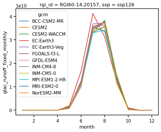
glacier_monthly_runoff = glacier.groupby(glacier['time.month']).mean()

glacier_annual_sum.plot(hue='gcm');

glacier_monthly_runoff.plot(hue='gcm');

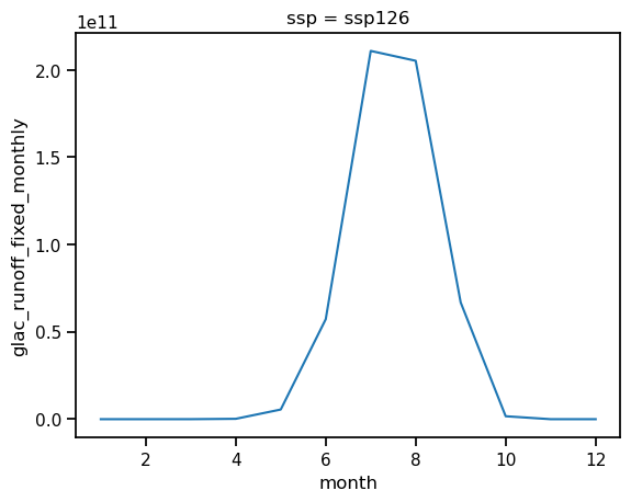
Or one can select all glaciers but average over the GCMS:

all_glaciers_gcm_avg = ds_rounce_ssp126.glac_runoff_fixed_monthly.sum(dim='rgi_id').mean(dim='gcm')
all_glaciers_gcm_avg_annual = all_glaciers_gcm_avg.resample(time='AS').sum()
all_glaciers_gcm_avg_monthly_runoff = all_glaciers_gcm_avg.groupby(all_glaciers_gcm_avg['time.month']).mean()

all_glaciers_gcm_avg_annual.plot();

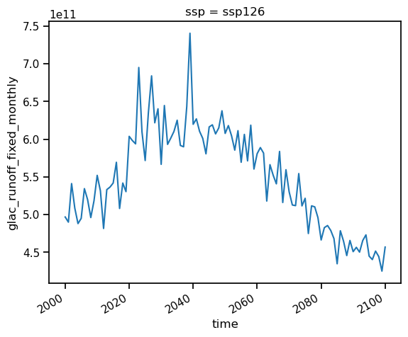
all_glaciers_gcm_avg_monthly_runoff.plot();

Running OGGM for a list of glaciers

357 glaciers might take too much time to run on classroom! So we select only the largest glaciers here:

rgi_df_sel_more = rgi_df_sel.loc[rgi_df_sel['Area'] > 5]
len(rgi_df_sel_more)

7

# OGGM options
oggm.cfg.initialize(logging_level='WARNING')
oggm.cfg.PATHS['working_dir'] = 'WaterResources-Proj-Astore'
oggm.cfg.PARAMS['store_model_geometry'] = True
oggm.cfg.PARAMS['dl_verify'] = False
oggm.cfg.PARAMS['use_multiprocessing'] = True  # Important!

2023-03-23 08:49:24: oggm.cfg: Reading default parameters from the OGGM `params.cfg` configuration file.

2023-03-23 08:49:24: oggm.cfg: Multiprocessing switched OFF according to the parameter file.

2023-03-23 08:49:24: oggm.cfg: Multiprocessing: using all available processors (N=8)

2023-03-23 08:49:24: oggm.cfg: PARAMS['store_model_geometry'] changed from `False` to `True`.

2023-03-23 08:49:24: oggm.cfg: PARAMS['dl_verify'] changed from `True` to `False`.

2023-03-23 08:49:24: oggm.cfg: Multiprocessing switched ON after user settings.

base_url = 'https://cluster.klima.uni-bremen.de/~oggm/gdirs/oggm_v1.6/L3-L5_files/2023.1/elev_bands/W5E5_spinup'
gdirs = workflow.init_glacier_directories(rgi_df_sel_more, from_prepro_level=5, prepro_border=160, prepro_base_url=base_url)

2023-03-23 08:49:24: oggm.workflow: init_glacier_directories from prepro level 5 on 7 glaciers.

2023-03-23 08:49:24: oggm.workflow: Execute entity tasks [gdir_from_prepro] on 7 glaciers

gdirs now contain 7 glaciers

len(gdirs)

7

Climate projections data

Before we run our future simulation we have to process the climate data for the glacier. We are using the bias-corrected projections from the Inter-Sectoral Impact Model Intercomparison Project (ISIMIP). They are offering climate projections from CMIP6 (the basis for the IPCC AR6) but already bias-corrected to our glacier grid point. Let’s download them:

# you can choose one of these 5 different GCMs:
# 'gfdl-esm4_r1i1p1f1', 'mpi-esm1-2-hr_r1i1p1f1', 'mri-esm2-0_r1i1p1f1' ("low sensitivity" models, within typical ranges from AR6)
# 'ipsl-cm6a-lr_r1i1p1f1', 'ukesm1-0-ll_r1i1p1f2' ("hotter" models, especially ukesm1-0-ll)
from oggm.shop import gcm_climate
member = 'mri-esm2-0_r1i1p1f1' 

# Download the three main SSPs
for ssp in ['ssp126', 'ssp370','ssp585']:
    # bias correct them
    workflow.execute_entity_task(gcm_climate.process_monthly_isimip_data, gdirs, 
                                 ssp = ssp,
                                 # gcm member -> you can choose another one
                                 member=member,
                                 # recognize the climate file for later
                                 output_filesuffix=f'_ISIMIP3b_{member}_{ssp}'
                                 );

2023-03-23 08:49:25: oggm.workflow: Execute entity tasks [process_monthly_isimip_data] on 7 glaciers

2023-03-23 08:49:26: oggm.workflow: Execute entity tasks [process_monthly_isimip_data] on 7 glaciers

2023-03-23 08:49:28: oggm.workflow: Execute entity tasks [process_monthly_isimip_data] on 7 glaciers

Projection run

With the climate data download complete, we can run the forced simulations:

for ssp in ['ssp126', 'ssp370', 'ssp585']:
    rid = f'_ISIMIP3b_{member}_{ssp}'
    workflow.execute_entity_task(tasks.run_with_hydro, gdirs,
                             run_task=tasks.run_from_climate_data, ys=2020,
                             # use gcm_data, not climate_historical
                             climate_filename='gcm_data',
                             # use the chosen scenario
                             climate_input_filesuffix=rid,
                             # this is important! Start from 2020 glacier
                             init_model_filesuffix='_spinup_historical',
                             # recognize the run for later
                             output_filesuffix=rid,
                             # add monthly diagnostics
                             store_monthly_hydro=True);

2023-03-23 08:49:30: oggm.workflow: Execute entity tasks [run_with_hydro] on 7 glaciers

2023-03-23 08:49:32: oggm.workflow: Execute entity tasks [run_with_hydro] on 7 glaciers

2023-03-23 08:49:33: oggm.workflow: Execute entity tasks [run_with_hydro] on 7 glaciers

Combine the data

For this we use the OGGM utility functions compile_*:

ds_historical = utils.compile_run_output(gdirs, input_filesuffix='_spinup_historical')

2023-03-23 08:49:35: oggm.utils: Applying global task compile_run_output on 7 glaciers

2023-03-23 08:49:35: oggm.utils: Applying compile_run_output on 7 gdirs.

ssp = 'ssp126'
ds_oggm_ssp126 = utils.compile_run_output(gdirs, input_filesuffix=f'_ISIMIP3b_{member}_{ssp}')
ssp = 'ssp370'
ds_oggm_ssp370 = utils.compile_run_output(gdirs, input_filesuffix=f'_ISIMIP3b_{member}_{ssp}')
ssp = 'ssp585'
ds_oggm_ssp585 = utils.compile_run_output(gdirs, input_filesuffix=f'_ISIMIP3b_{member}_{ssp}')

2023-03-23 08:49:35: oggm.utils: Applying global task compile_run_output on 7 glaciers

2023-03-23 08:49:35: oggm.utils: Applying compile_run_output on 7 gdirs.

2023-03-23 08:49:35: oggm.utils: Applying global task compile_run_output on 7 glaciers

2023-03-23 08:49:35: oggm.utils: Applying compile_run_output on 7 gdirs.

2023-03-23 08:49:35: oggm.utils: Applying global task compile_run_output on 7 glaciers

2023-03-23 08:49:35: oggm.utils: Applying compile_run_output on 7 gdirs.

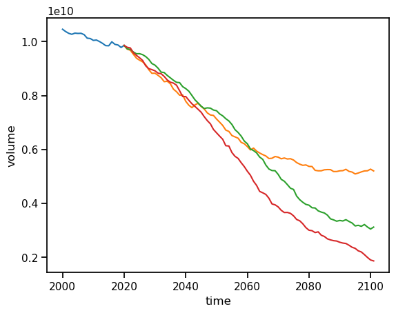
ds_historical.volume.sum(dim='rgi_id').sel(time=slice('2000', '2021')).plot();
ds_oggm_ssp126.volume.sum(dim='rgi_id').plot();
ds_oggm_ssp370.volume.sum(dim='rgi_id').plot();
ds_oggm_ssp585.volume.sum(dim='rgi_id').plot();

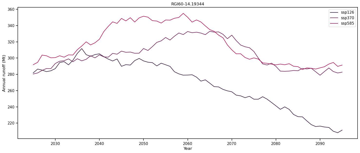
Plot the hydrological output

# Create the figure
f, ax = plt.subplots(figsize=(18, 7), sharex=True)
# Loop over all scenarios
for i, ssp in enumerate(['ssp126', 'ssp370', 'ssp585']):
    file_id = f'_ISIMIP3b_{member}_{ssp}'
    
    # This repeats the step above but hey
    ds = utils.compile_run_output(gdirs, input_filesuffix=f'_ISIMIP3b_{member}_{ssp}')
    ds = ds.sum(dim='rgi_id').isel(time=slice(0, -1))
        
    # Select annual variables
    sel_vars = [v for v in ds.variables if 'month_2d' not in ds[v].dims]
    # And create a dataframe
    df_annual = ds[sel_vars].to_dataframe()

    # Select the variables relevant for runoff.
    runoff_vars = ['melt_off_glacier', 'melt_on_glacier', 
                   'liq_prcp_off_glacier', 'liq_prcp_on_glacier']
    # Convert to mega tonnes instead of kg.
    df_runoff = df_annual[runoff_vars].clip(0) * 1e-9
    # Sum the variables each year "axis=1", take the 11 year rolling mean and plot it.
    df_roll = df_runoff.sum(axis=1).rolling(window=11, center=True).mean()
    df_roll.plot(ax=ax, label=ssp, color=sns.color_palette("rocket")[i])

ax.set_ylabel('Annual runoff (Mt)'); ax.set_xlabel('Year'); plt.title(gdirs[0].rgi_id); plt.legend();

2023-03-23 08:49:36: oggm.utils: Applying global task compile_run_output on 7 glaciers

2023-03-23 08:49:36: oggm.utils: Applying compile_run_output on 7 gdirs.

2023-03-23 08:49:36: oggm.utils: Applying global task compile_run_output on 7 glaciers

2023-03-23 08:49:36: oggm.utils: Applying compile_run_output on 7 gdirs.

2023-03-23 08:49:36: oggm.utils: Applying global task compile_run_output on 7 glaciers

2023-03-23 08:49:36: oggm.utils: Applying compile_run_output on 7 gdirs.

Let’s compare Rounce et al. (2023) data and OGGM for these 7 selected glaciers, GCM and SSP

OGGM first:

# Select the variables relevant for runoff.
runoff_vars = ['melt_off_glacier', 'melt_on_glacier', 
               'liq_prcp_off_glacier', 'liq_prcp_on_glacier']
# And create a dataframe
df_annual = ds_oggm_ssp126[sel_vars].sum(dim='rgi_id').isel(time=slice(0, -1)).to_dataframe()

# Select the variables relevant for runoff.
runoff_vars = ['melt_off_glacier', 'melt_on_glacier', 
               'liq_prcp_off_glacier', 'liq_prcp_on_glacier']
# Convert to mega tonnes instead of kg.
df_runoff = df_annual[runoff_vars].clip(0) * 1e-9

Then Rounce:

ds_rounce_ssp126_sel = ds_rounce_ssp126.sel(rgi_id=ds_oggm_ssp126.rgi_id, gcm='MRI-ESM2-0')
ds_rounce_ssp126_sel = ds_rounce_ssp126_sel.glac_runoff_fixed_monthly.sum(dim='rgi_id').resample(time='AS').sum() * 1e-9
ds_rounce_ssp126_sel['time'] = ds_rounce_ssp126_sel['time.year'] 

df_runoff.sum(axis=1).plot(label='OGGM');
ds_rounce_ssp126_sel.plot(label='Rounce et al.');
plt.ylabel('Annual runoff (Mt)'); plt.legend();

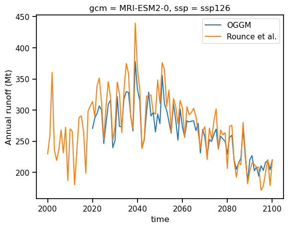
That’s very close! Often the projections are not so close though.