Mass balance gradients (MBG) and their influence on glacier flow

In the intro notebook we touched briefly on the mass balance gradient of a glacier. This is what we are going to take a closer look at now. If the concept of mass balance is completely new to you, have a short read about it here, up to the paragraph “So what is Glacier Mass Balance?”. In this notebook we will set up a few simple glaciers to further explore what characteristics of glaciers change with different mass balance gradients. We will also take a look at the topics of volume and response time.

Goals of this notebook:

• The student will be able to explain the terms:

  • Mass balance gradient,

  • Equilibrium state

  • Response time.

First, we have to import the relevant classes

from oggm_edu import MassBalance, GlacierBed, Glacier, GlacierCollection

Initialising the glacier

We start by setting up a simple glacier with a linear bedrock (see Getting started with OGGM Edu) to generate a starting point for our experiment.

# Bed
bed = GlacierBed(top=3400, bottom=1500, width=400)
# Mass balance
mass_balance = MassBalance(ela=3000, gradient=4)
# Glacier
glacier = Glacier(bed=bed, mass_balance=mass_balance)

Changing the mass balance gradient (MBG)

The MBG is defined as the change of the mass balance with altitude ¹. It depends strongly on the climate at the glacier ².

Let’s take a look at the effects of the MBG by creating a few glaciers with different gradients. In the intro notebook our glacier had a gradient of 4 mm/m so lets add a glacier with a weaker gradient and one with a stronger gradient.

We will again make use of the GlacierCollection to quickly progress and visualise the glaciers.

collection = GlacierCollection()
# Fill the collection. This time we change the attributes on creation.
collection.fill(glacier, n=3, attributes_to_change=
                {'gradient':[0.3, 4, 15]}
               )

Creating a complex mass balance profile

It is also possible to create a more complex mass balance profile. This is achieved by passing a list of gradients, and another list with the altitude of the breakpoints between them.

# Add complex mb profile
complex_mb = MassBalance(ela=3000, gradient=[3, 7, 10, 15],
                         breakpoints=[2700, 2250, 1800])
glacier_complex_mb = Glacier(bed=bed, mass_balance=complex_mb)

# Add the new glacier to the collection.
collection.add(glacier_complex_mb)

# Progress collection to the same year.
collection.progress_to_year(300)

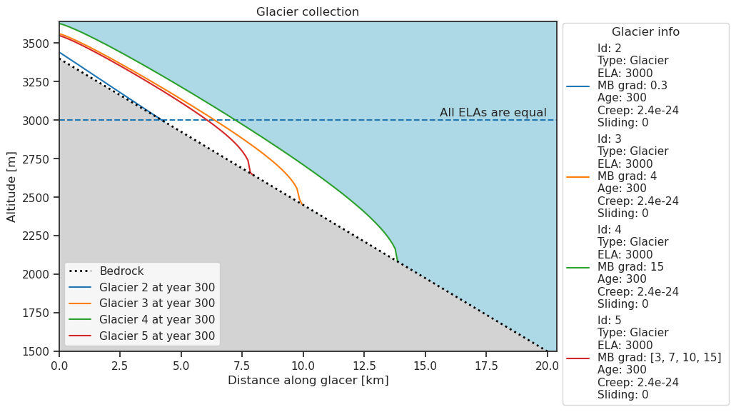
collection.plot()

collection.plot_mass_balance()

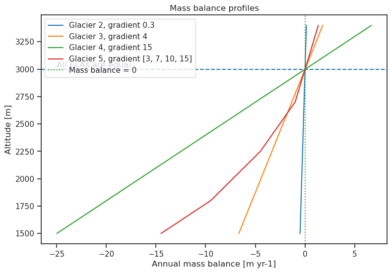
A stronger mass balance gradient (flatter line in plot above) implies a larger change of the mass balance with altitude. We can see this in the plot above: The annual mass balance hardly changes with altitude for the glacier with the weakest mass balance gradient (blue) while there is a considerable difference between the top and bottom annual mass balance for the glacier with the strongest mass balance gradient (green).

This in turn affects the growth of the glacier. A strong mass balance gradient implies that more ice is added to the accumulation zone while more ice is removed from the ablation zone each year compared to a glacier with a weaker gradient. This results in a greater ice flux and the glacier thus grows faster. This is why the glacier with the strongest gradient exhibits the largest growth during our experiments (Green glacier in Collection plot above).

What do you think: where do we find glaciers with high MBGs? Click for details

You will find a short explanation in this paragraph on AntarcticGlaciers.org.

Equilibrium state

Glaciers change their geometry as a way to adapt to the climate³. If the accumulation increases, the glacier will grow further down below the ELA to increase the ablation. Similarly, if the temperature rises and the ablation increases, the glacier length will decrease. If the climate remains constant for a long enough time, glaciers will reach an equilibrium state with its climate, where the accumulation = ablation ⁴.

With this in mind, we will take a look at how fast our glaciers, with different gradients, reach this state and compare their shapes:

# We reset the collection.
collection = GlacierCollection()
# Fill the collection. This time we change the attributes on creation.
collection.fill(glacier, n=3, attributes_to_change=
                {'gradient':[0.3, 4, 15]}
               )

# First we progress the glaciers to equilibrium.
collection.progress_to_equilibrium()

# Plot it
collection.plot()

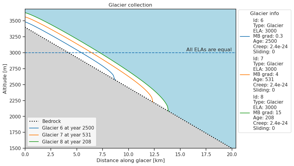
The different glaciers reach their equilibrium state after a different number of years. What does the figure show us? Which glacier is the thickest and longest? Let’s look at specific numbers:

collection

	Id	Type	Age	Length [m]	Area [km2]	Volume [km3]	Max ice thickness [m]	Max ice velocity [m/yr]	AAR [%]	Response time [yrs]	...	Basal sliding	Bed type	Top [m]	Bottom [m]	Width(s) [m]	Length [km]	ELA [m]	Original ELA [m]	Temperature bias [C]	Gradient [mm/m/yr]
Glacier
1	6	Glacier	2500	8700.0	3.48	0.376764	119.836207	6.25951	63.218391	NaN	...	0	Linear bed with a constant width	3400	1500	400	20.0	3000	3000	0	0.3
2	7	Glacier	531	12300.0	4.92	0.935159	214.228472	64.34719	52.845528	NaN	...	0	Linear bed with a constant width	3400	1500	400	20.0	3000	3000	0	4.0
3	8	Glacier	208	13800.0	5.52	1.418343	291.286530	215.60993	52.173913	NaN	...	0	Linear bed with a constant width	3400	1500	400	20.0	3000	3000	0	15.0

3 rows × 21 columns

The glacier with the strongest gradient reaches the equilibrium state first. This is also the largest and longest glacier.

Response time

The glacier response time is the period of time a glacier needs to adjust its geometry to changes in mass balance caused by climate change and reach a new equilibrium state. There are a some different definitions for its calculation, OGGM-Edu use the definition from Oerlemans (see formula below) ⁵.

A OGGM-Edu glacier has an attribute .response_time which is calculated based on difference between the last two equilibrium states in the glacier history. So far we’ve only showed you how to progress a glacier to equilibrium, but not how to leave it and reach a second one. This will be the first step to getting the response time of a glacier.

We use the glacier from the start of the notebook.

# Check the state, everything should be zero/nan here.
glacier

Attribute
Id	1
Type	Glacier
Age	0
Length [m]	0.0
Area [km2]	0.0
Volume [km3]	0.0
Max ice thickness [m]	0.0
Max ice velocity [m/yr]	None
AAR [%]	NaN
Response time [yrs]	NaN
Creep (Glen A)	2.4e-24
Basal sliding	0

First we progress the glacier to equilibrium

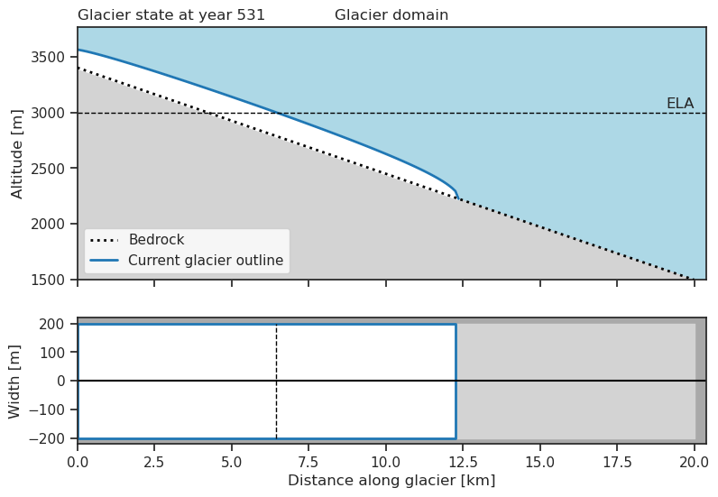
glacier.progress_to_equilibrium()

glacier.plot()

We can access the stored equilibrium states of a glacier

glacier.eq_states

{531: 3000}

Now we want to set up a climate change scenario for the glacier. This is easily done with the .add_temperature_bias method. This method takes a desired temperature bias (\(+/-\)) and a duration, which specifies how long it will take for the glacier to reach the climate state. For instance, if we set the bias to 1. and the duration to 50, it will take 50 years for the climate to become 1 degree warmer.

When a glacier has a climate change scenario the progress_ methods will internally work a little bit differently, but this is not anything you will notice.

Since we are purely interested in the response of the glacier, we create a climate change scenario with the duration of 1 year.

# Add a climate change scenario
glacier.add_temperature_bias(bias=1., duration=1)

How does the ELA respond if we raise the temperature? Click for a hint

Raising the temperature will increase the size of the ablation area of the glacier, and thus the ELA will increase.

# We can then progress the glacier to equilibrium again
glacier.progress_to_equilibrium()

glacier.plot()

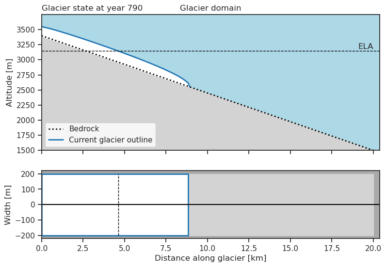
glacier.eq_states

{531: 3000, 790: 3150.0}

The next step is to calculate the response times for our glaciers. One could think that it is as simple as looking at the years above and do a simple subtraction. However this is not the case! In reality the rate at which a glacier changes is ever decreasing and a complete equilibrium state is never really achieved. Because of this the response time is considered the time it has taken the glacier to complete most of the adjustment, more specifically all but a factor of \(1/e\).

For numerical models like our glaciers it is common to use the volume response time, from Oerlemans ⁵:

\[ \tau = t \left(V=V_2 - \frac{V_2 - V_1}{e}\right) \]

where \(V_1\) and \(V_2\) corresponds to the glacier volume at the initial and new equilibrium state respectively.

Luckily this is done by our glacier object, so we can just take look at the .response_time attribute

glacier.response_time

69.0

or just look at the representation

glacier

Attribute
Id	1
Type	Glacier
Age	790
Length [m]	8900.0
Area [km2]	3.56
Volume [km3]	0.58815
Max ice thickness [m]	187.240744
Max ice velocity [m/yr]	64.34719029759603
AAR [%]	51.685393
Response time [yrs]	69.0
Creep (Glen A)	2.4e-24
Basal sliding	0

Now that we have introduced the concept of response time we can apply it and see how the different mass balance gradients affect the response time. For this we need a new collection.

# Bed
bed = GlacierBed(top=3400, bottom=1500, width=400)
# Mass balance
mass_balance = MassBalance(ela=3000, gradient=4)
# Glacier
glacier = Glacier(bed=bed, mass_balance=mass_balance)

collection = GlacierCollection()
# Fill the collection. This time we change the attributes on creation.
collection.fill(glacier, n=3, attributes_to_change=
                {'gradient':[1, 4, 15]}
               )

collection.progress_to_equilibrium()

collection

	Id	Type	Age	Length [m]	Area [km2]	Volume [km3]	Max ice thickness [m]	Max ice velocity [m/yr]	AAR [%]	Response time [yrs]	...	Basal sliding	Bed type	Top [m]	Bottom [m]	Width(s) [m]	Length [km]	ELA [m]	Original ELA [m]	Temperature bias [C]	Gradient [mm/m/yr]
Glacier
1	10	Glacier	1396	11100.0	4.44	0.617531	156.657721	18.163011	53.153153	NaN	...	0	Linear bed with a constant width	3400	1500	400	20.0	3000	3000	0	1
2	11	Glacier	531	12300.0	4.92	0.935159	214.228472	64.347190	52.845528	NaN	...	0	Linear bed with a constant width	3400	1500	400	20.0	3000	3000	0	4
3	12	Glacier	208	13800.0	5.52	1.418343	291.286530	215.609930	52.173913	NaN	...	0	Linear bed with a constant width	3400	1500	400	20.0	3000	3000	0	15

3 rows × 21 columns

We then have to set up a climate change scenario for the glaciers in the collection

# Same scenario for all the glaciers.
collection.glaciers[0].add_temperature_bias(bias=1., duration=1)
collection.glaciers[1].add_temperature_bias(bias=1., duration=1)
collection.glaciers[2].add_temperature_bias(bias=1., duration=1)

# Progress to equilibrium again
collection.progress_to_equilibrium()

collection

	Id	Type	Age	Length [m]	Area [km2]	Volume [km3]	Max ice thickness [m]	Max ice velocity [m/yr]	AAR [%]	Response time [yrs]	...	Basal sliding	Bed type	Top [m]	Bottom [m]	Width(s) [m]	Length [km]	ELA [m]	Original ELA [m]	Temperature bias [C]	Gradient [mm/m/yr]
Glacier
1	10	Glacier	2033	8000.0	3.20	0.378810	134.826892	18.163011	51.250000	227.0	...	0	Linear bed with a constant width	3400	1500	400	20.0	3150.0	3000	1.0	1
2	11	Glacier	790	8900.0	3.56	0.588150	187.240744	64.347190	51.685393	69.0	...	0	Linear bed with a constant width	3400	1500	400	20.0	3150.0	3000	1.0	4
3	12	Glacier	319	10100.0	4.04	0.913352	256.795193	215.609930	52.475248	24.0	...	0	Linear bed with a constant width	3400	1500	400	20.0	3150.0	3000	1.0	15

3 rows × 21 columns

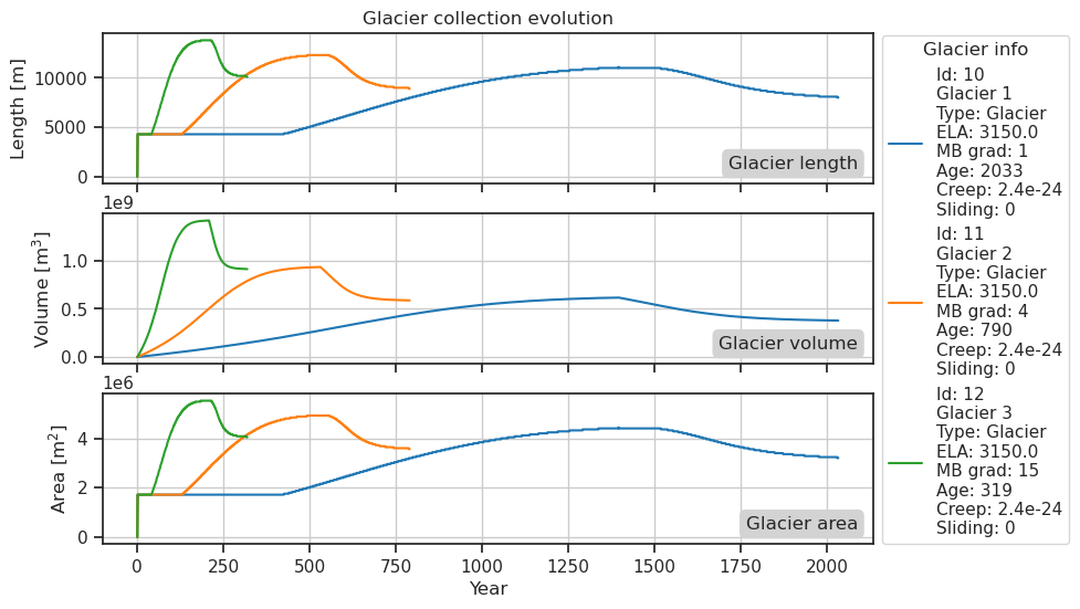
collection.plot_history()

We can also look at the state history for one of the glaciers

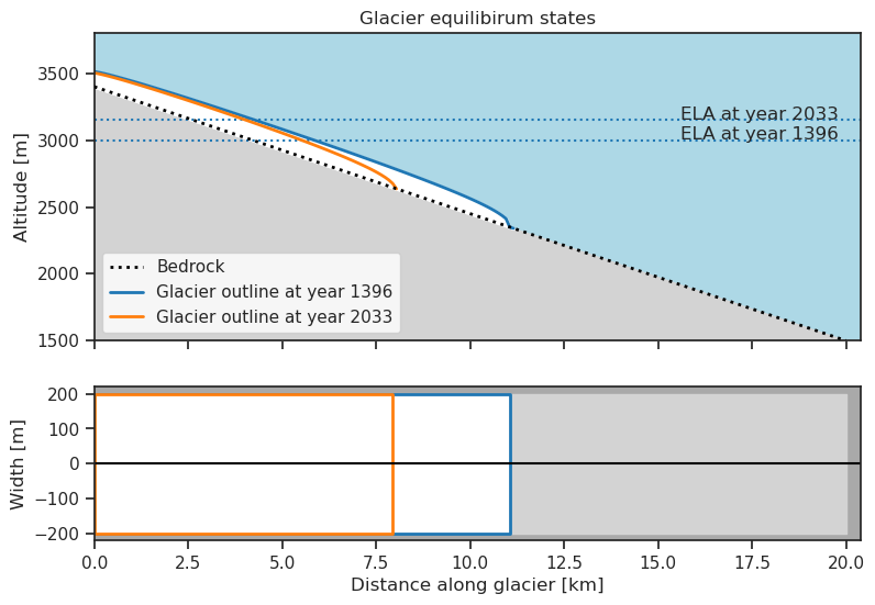
# Plots the glacier outline for the equilibrium states.
collection.glaciers[0].plot_state_history(eq_states=True)

The glacier with weakest MBG need the longest time to adjust to a changed climate compared to the other glaciers. On the other hand, the glacier with the strongest gradient only needs a around two decades to adjust its shape to the new climate (A real world example: Franz Josef glacier in New Zealand⁶)⁷. The response time of glaciers with weak gradients is in reality much longer than 200 years, actually closer to 2000 years.

Why does the MBG change response time of a glacier? What other factors except for the MBG do you think affect the response time of a glacier? Click me for a hint

The MBG affects the how fast the glacier will flow and in turn how fast the shape and size of the glacier can change. In general, we have to consider that the response time also depends on other features like the glacier-type, size, bed slope and average surface elevation.

References

¹ Rasmussen, L. A., & Andreassen, L. M. (2005). Seasonal mass-balance gradients in Norway. Journal of Glaciology, 51(175), 601-606.

² Oerlemans, J., & Fortuin, J. P. F. (1992). Sensitivity of glaciers and small ice caps to greenhouse warming. Science, 258(5079), 115-117.

³ Oerlemans, J. (2001). Glaciers and climate change. CRC Press.

⁴ Encyclopedia of snow, ice and glaciers, V.P. Singh, P. Singh, and U.K. Haritashya, Editors. 2011, Springer: Dordrecht, The Netherlands. p. 245-256.

⁵ Oerlemans, J. (1997). Climate sensitivity of Franz Josef Glacier, New Zealand, as revealed by numerical modeling. Arctic and Alpine Research, 29(2), 233-239.

⁶ Anderson, B., Lawson, W., & Owens, I. (2008). Response of Franz Josef Glacier Ka Roimata o Hine Hukatere to climate change. Global and Planetary Change, 63(1), 23-30.

⁷ Cuffey, K.M. & Paterson, W.S.B. The Physics of Glaciers, 4th edition, 704 (Academic Press, 2010).

What’s next?

Back to the table of contents