Glaciers as a low-pass filter of climate variations#
In a previous notebook we have talked about the response time of a glacier and how it takes some time for the glacier to respond to changes in its climate. In this notebook we are going to investigate this delayed response further by looking at how glaciers acts as a smoothing filter (low-pass) on variations in the climate forcing.
We will do this by introducing some, for you, new functionality of the OGGM-Edu classes which enables you to assign random, and custom, future temperature biases to the mass balance of your glacier.
First we have to import the minimal set of classes for working with OGGM-Edu glaciers.
from oggm_edu import GlacierBed, MassBalance, Glacier
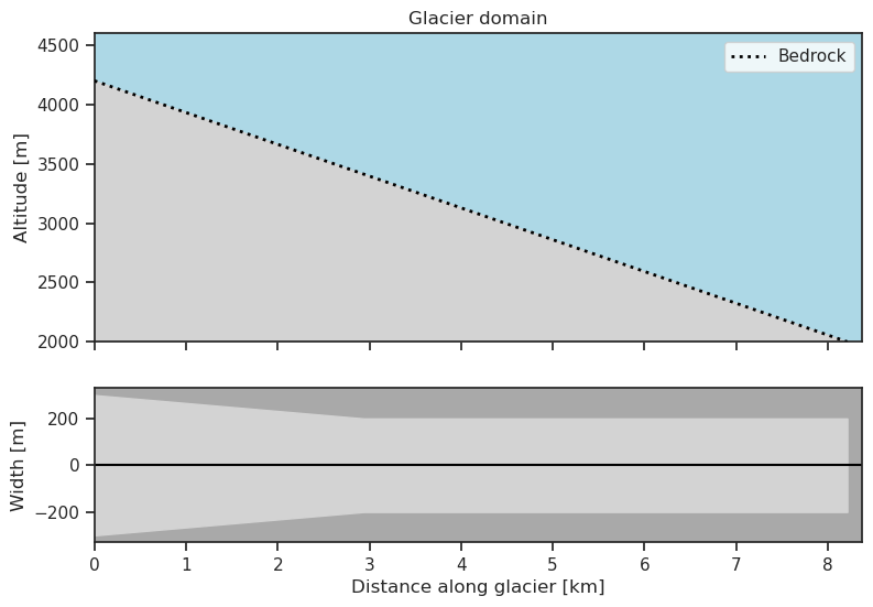
Then we create a bed. For these examples we can use a fairly simply bed with a single slope. However, feel free to change this as you like.
# Lets create a relatively simple bed.
bed = GlacierBed(widths=[600, 400, 400],
                 altitudes=[4200, 3400, 2000],
                 slopes=15)
bed.plot()
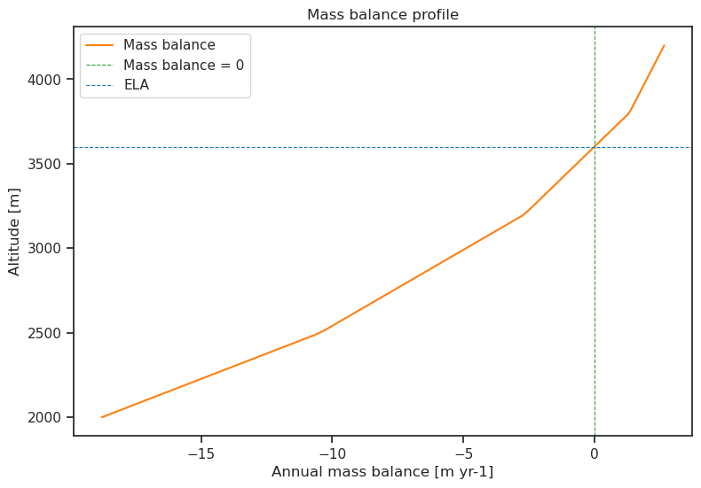
Next step is the mass balance. We create a slightly more realistic mass balance profile with a few different gradients.
# A mass balance with the ela at 3600 m. and 4 gradients.
mass_balance = MassBalance(ela=3600,
                           gradient=[3, 6, 10, 15],
                           breakpoints=[3800, 3200, 2500])
Now we are ready to create the glacier.
glacier = Glacier(bed=bed, mass_balance=mass_balance)
Let’s take a look at the mass balance profile.
glacier.plot_mass_balance()
Adding a random climate#
Before we start progressing the glacier assign a random climate to the future of the glacier. Random in this case means that the temperature bias of our glacier will vary randomly from year to year between values specified by us. Internally this has the effect that the ELA of our glacier changes up and down.
We assign a random climate through.add_random_climate(duration, temperature_range), a method of the Glacier object.
duration specifies how long the random climate should last, while temperature_range lets the user specify between what temperatures the climate should vary.
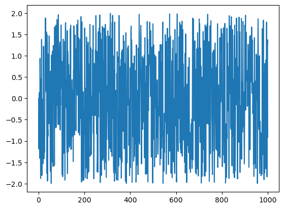
# Lets add a random climate for a 1000 years, varying between -2 and 2 degrees.
glacier.add_random_climate(duration=1000, temperature_range=[-2., 2.])
We can take a look at the random climate through the temperature_bias_series attribute of the MassBalance.
# This is a pandas dataframe.
glacier.mass_balance.temp_bias_series
| year | bias | |
|---|---|---|
| 0 | 0.0 | 0.000000 |
| 1 | 1.0 | -1.184740 |
| 2 | 2.0 | -0.385436 |
| 3 | 3.0 | 0.136106 |
| 4 | 4.0 | -0.735251 |
| ... | ... | ... |
| 996 | 996.0 | -0.949218 |
| 997 | 997.0 | -1.841776 |
| 998 | 998.0 | 1.187378 |
| 999 | 999.0 | 1.375924 |
| 1000 | 1000.0 | -0.917359 |
1001 rows × 2 columns
And also quickly plot it. This will be pretty messy.
glacier.mass_balance.temp_bias_series.bias.plot();
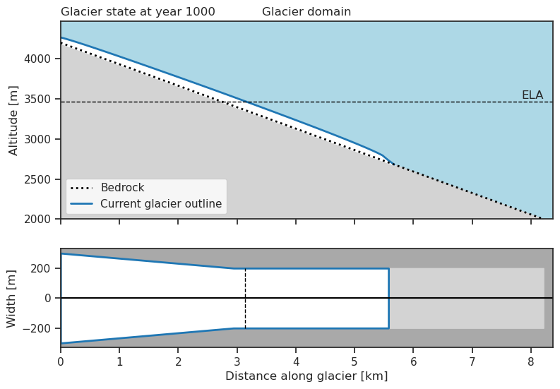
Now we can progress the glacier as usual.
# Progress the glacier to year 1000.
glacier.progress_to_year(1000)
glacier.plot()
A look at the history#
We plot the history of the glacier length, volume and area with the .plot_history() method.
We can also plot the temperature bias history by passing True to the show_bias argument.
glacier.plot_history(show_bias=True)
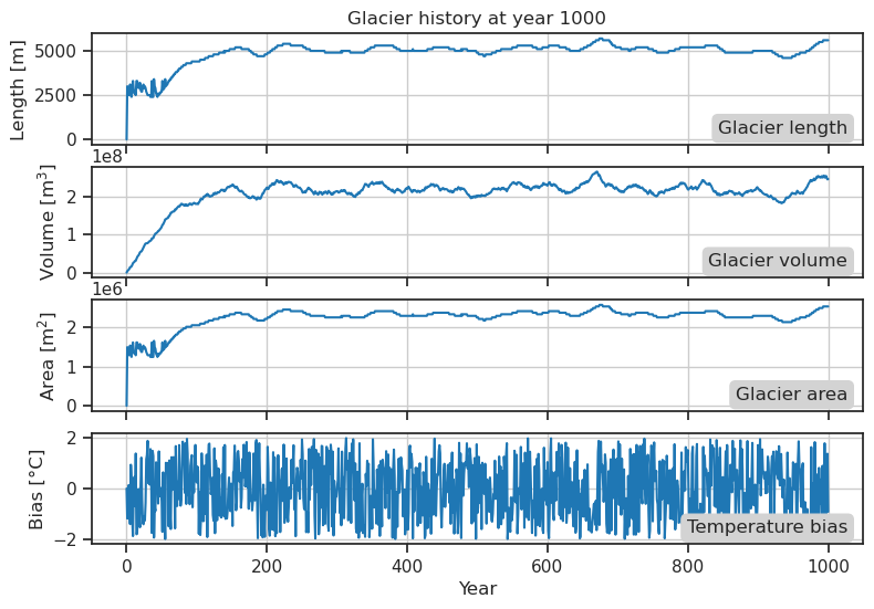
Since the random climate is just random, it is difficult to distinguish any similarities between the noisy bias and the glacier history.
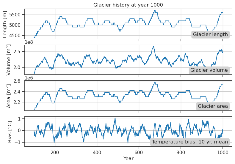
However, we can smooth the bias by providing a window size to the window argument.
This will perform a rolling mean on the temperature bias series before plotting it.
Here we also specify a time frame to plot in order to get a closer look at the data. By doing this we shrink the range of the y-axis, enhancing the fluctuations in the glacier history.
Try executing the cell below with different window sizes and try to find the size which represent the smoothing that the glacier have on the climate. [Click for a hint]
With a window size around 30-40 years, the bias begins to exhibit patterns similar to the glacier history.
# Smooth the bias so that it resembles the history of the glacier attributes.
glacier.plot_history(show_bias=True, window=10,
                     time_range=[100, 1000])
Creating a custom climate#
It is possible to create a completely custom climate for the glacier.
This is done by creating an array of bias values and assigning it to the .temp_bias_series attribute.
The easiest way to do this is by using one, or a combination, of the numpy-methods generating arrays.
import numpy as np
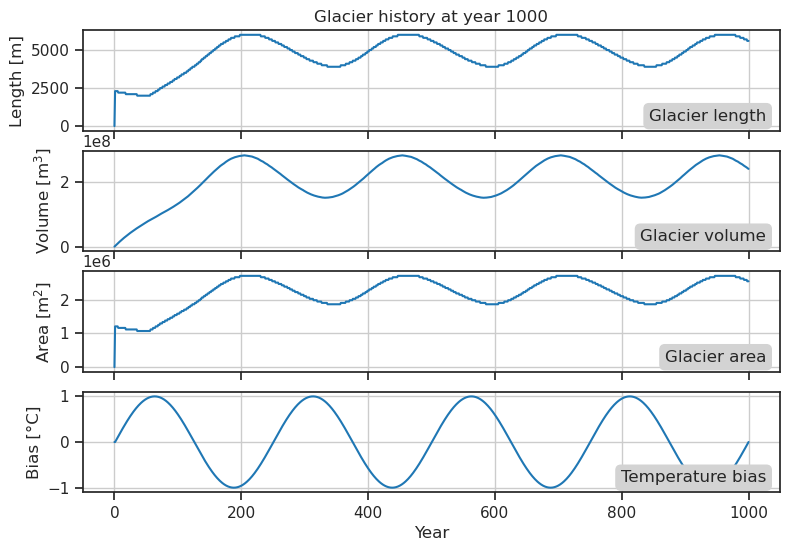
For this exercise we will create a sinusoidal bias, not because it is very realistic but to show one example of how one can use convenient functions to generate the values. You can essentially use any function returning an array of floats, or do it manually, to create the bias series of your imagination.
# How many cycles and years do we want?
n_cycles = 4
# 1000 years, we add 1 since last number is not included.
n_years = 1000
# Radians.
rads = np.linspace(0, n_cycles * 2 * np.pi, n_years)
# Create the sinus waves.
bias_data = np.sin(rads)
We reset the glacier before adding the new climate, to start fresh.
glacier.reset()
Then we can assign the bias_data to the .temp_bias_series.
glacier.mass_balance.temp_bias_series = bias_data
Progress the glacier as usual.
glacier.progress_to_year(1000)
Take a look at the history of the glacier
glacier.plot_history(show_bias=True)
It is also possible to add a future climate to a glacier that already has some history.
To start over, we first reset the glacier, then we add a linear trend and progress to the end of the climate data.
glacier.reset()
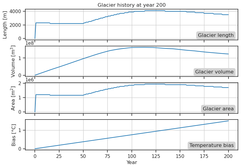
glacier.add_temperature_bias(bias=1.5, duration=200)
glacier.progress_to_year(200)
glacier.plot_history(show_bias=True)
We can then assign more data to the future climate, just as easy as before. we now want a sinus-wave that oscillates around the current temperature bias.
# How many cycles and years do we want?
n_cycles = 4
# 1000 years, we add 1 since last number is not included.
n_years = 1000
# Radians.
rads = np.linspace(0, n_cycles * 2 * np.pi, n_years)
# Create the sinus wave and add the current temperature bias.
bias_data = np.sin(rads) + glacier.mass_balance.temp_bias
Assign it to the .temp_bias_series.
Internally this will append it to the series that already exists.
glacier.mass_balance.temp_bias_series = bias_data
# We progress to year 1154, the current age + 1000.
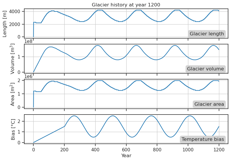
glacier.progress_to_year(1200)
glacier.plot_history(show_bias=True)
Adding noise to clean data#
Until now, we have either created a completely random climate or very clean and predictable trends. The next step is, of course, to combine the methods to create trends that also have some random variability to them.
We will demonstrate this by manually creating a linear trend and then adding some noise to it.
glacier.reset()
# Create a linear trend, from 0 to 2 degrees in 200 years
trend = np.linspace(0, 2, 200)
# And some noise. Interannual variability of +- 2 degrees
noise = (np.random.rand(200) * 4) - 2
# Add the noise to the trend
bias = trend + noise
We first add only some noise to get a noisy “spin up” of the glacier.
noise = (np.random.rand(500) * 4) - 2
glacier.mass_balance.temp_bias_series = noise
Then lets add the trend, remember that this will append to the future of the climate.
glacier.mass_balance.temp_bias_series = bias
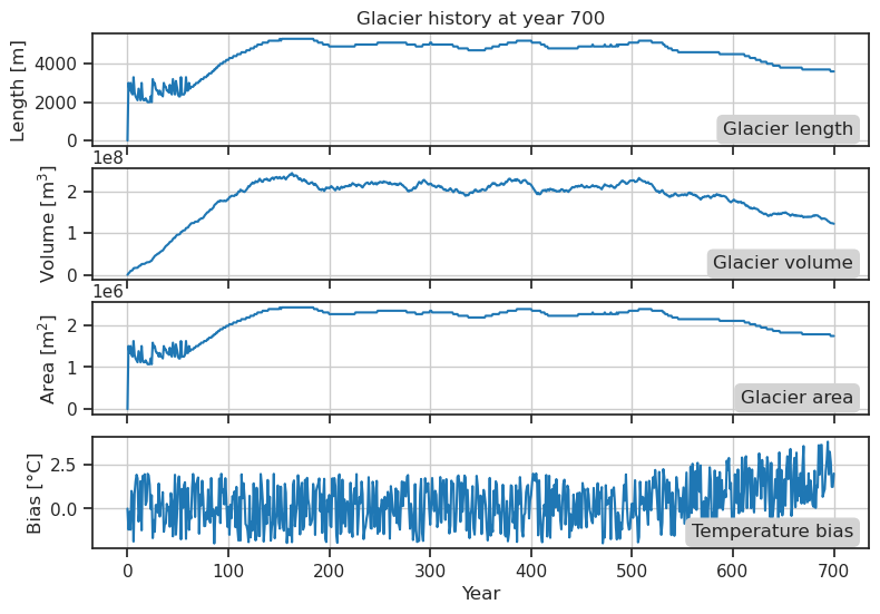
Progress to the end of the climate data.
glacier.progress_to_year(700)
glacier.plot_history(show_bias=True)
Conveniently, the .add_temperature_bias has an argument which adds noise to the trend.
glacier.reset()
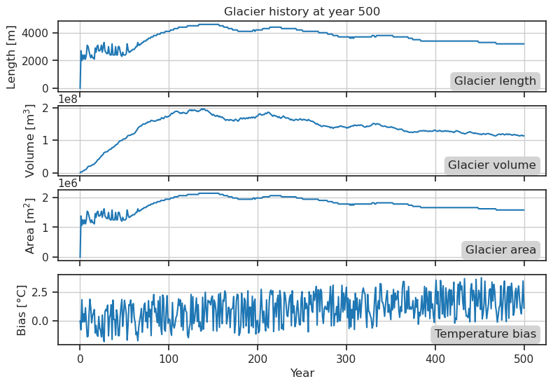
glacier.add_temperature_bias(bias=2., duration=500, noise=(-2, 2))
glacier.progress_to_year(500)
glacier.plot_history(show_bias=True)
Now you should have the tools to create your own climates for OGGM-Edu glaciers and see how they filter the climate.