Ice on an incline#
This activity can be run by students after a live experiment with “glacier goo” used on various slopes. In this notebook, we use a numerical simulation to study the difference in ice flow between bed of various slopes.
First, we set up the tools that we will use. You won’t need to modify these.
# import special helps from the OGGM-Edu package
from oggm_edu import MassBalance, GlacierBed, Glacier, GlacierCollection
The essentials#
Now we set up our first slope and tell the model that we want to study a glacier there. We will keep things simple: a constant slope, constant valley width, and simple formulation for adding and removing ice according to altitude.
The glacier bed#
We will use a helper function to create a simple bed with a constant slope. This requires as input a top and bottom altitude, and a width.
# define glacier slope and how high up it is
top_elev = 3400 # m, the peak elevation
bottom_elev = 1500 # m, the elevation at the bottom of the glacier
We have to decide how wide our glacier is. For now, we will use a default RectangularBedFlowline shape with an initial_width width of 300 m. The “rectangular” cross-sectional shape means that the glacial “valley” walls are straight and the width w is the same throughout:
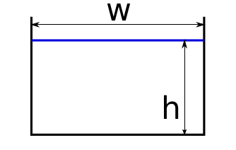
In this image, the black lines signify the walls of the “valley”. The blue line shows the surface of the glacier.
What do you think *h* means in the picture? Click for details
If you are interested, you can read more about glacier bed shapes in the OGGM documentation.
We set up a glacier bed with the specified geometry:
bed_width = 300  # m, the constant width of the rectangular valley
bed_slope = 10  # degrees, the slope of the bed
bed = GlacierBed(top=top_elev, bottom=bottom_elev, width=bed_width, slopes=bed_slope)
Let’s plot the bed to make sure that it looks like we expect. The GlacierBed object has a built in method for this which provide us with a side and top-down view of the glacier domain.
bed.plot()
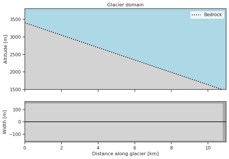
Check out the glacier bed length. How do you think that the length is computed out of the parameters above? Click for details
Internally, the GlacierBed will compute the length out of the top and bottom height and a little bit of trigonometry.
We have now defined an object called GlacierBed and assigned it to the variable bed, which stores all the information about the bed geometry that the model uses.
# This gives us some statistics about the bed.
bed
| GlacierBed | |
|---|---|
| Bed type | Linear bed with a constant width |
| Top [m] | 3400 |
| Bottom [m] | 1500 |
| Width(s) [m] | [300] |
| Length [km] | 10.775435 |
Notice that bed does not include any information about the ice. So far we have only set up a valley. We have defined its slope, its width, its transverse shape - the geometry of the habitat where our glacier will grow. Now we want to add the climate processes that will put ice into that habitat.
Adding the ice#
Now we want to add ice to our incline and make a glacier. Glaciologists describe the amount of ice that is added or removed over the entire surface of the glacier as the “mass balance”. Here’s an illustration from the OGGM-edu website:
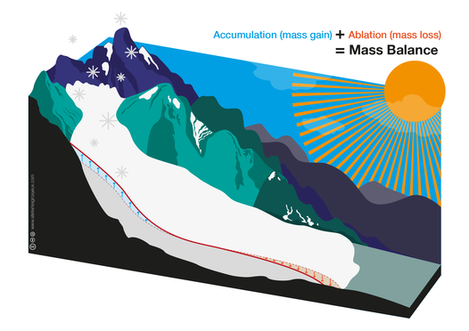
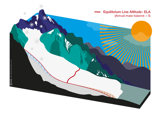
A linear mass balance is defined by an equilibrium line altitude (ELA) and a mass balance gradient with altitude (in [mm m \(^{- 1}\)]). Above the ELA, we add ice (from snow) and below the line we remove ice (melting it). We will learn more about this in the accumulation and ablation notebook.
# ELA at 3000m a.s.l., gradient 4 mm m-1
ELA = 3000 # equilibrium line altitude in meters above sea level
altgrad = 4 # altitude gradient in mm/m
mb_model = MassBalance(ELA, gradient=altgrad)
mb_model
| MassBalance | |
|---|---|
| ELA [m] | 3000 |
| Original ELA [m] | 3000 |
| Temperature bias [C] | 0 |
| Gradient [mm/m/yr] | [4] |
The mass balance model mb_model gives us the mass balance for any altitude we want. We will plot it below.
Glacier initialisation#
We can now take our bed and the mass balance and create a glacier which we can then perform experiments on.
# Initialise the glacier
glacier = Glacier(bed=bed, mass_balance=mb_model)
Similarly to the bed, the Glacier object is storing some information that we can recover just by calling it:
glacier
| Attribute | |
|---|---|
| Id | 1 |
| Type | Glacier |
| Age | 0 |
| Length [m] | 0.0 |
| Area [km2] | 0.0 |
| Volume [km3] | 0.0 |
| Max ice thickness [m] | 0.0 |
| Max ice velocity [m/yr] | None |
| AAR [%] | NaN |
| Response time [yrs] | NaN |
| Creep (Glen A) | 2.4e-24 |
| Basal sliding | 0 |
Since we just created the glacier, there’s still no ice! We need some time for ice to accumulate. For this, the mass balance is the relevant process:
glacier.plot_mass_balance()
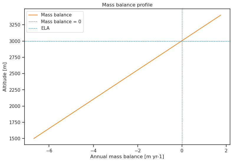
What did you notice in the graph? What are the axes? At what altitudes is ice added to the glacier (positive mass balance)? At what altitudes does ice melt?
Running the numerical model#
When we did our experiments in the laboratory, we had a slope and some material to pour our “glacier”. We also decided how long to let the goo flow – that is, the “runtime” of our experiment. Setting up our glacier model on the computer is very similar. We have gathered our bed geometry (bed), our mass balance (mb_model), and now we will tell the model how long to run (runtime).
First we run the model for one year:
# We want to progress the glacier by a given time.
runtime = 1
glacier.progress_to_year(runtime)
Let’s take a look. The Glacier object also has a built-in method for us to plot.
glacier.plot()
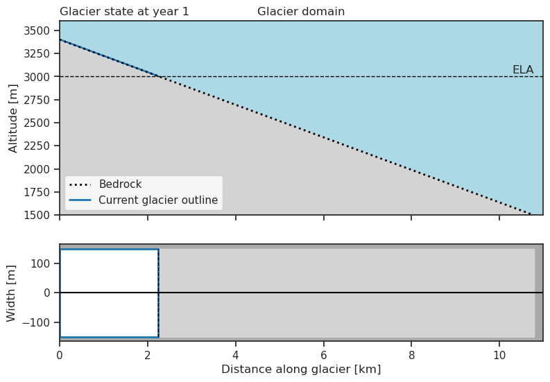
Here we can see that there is a very thin cover of ice from the top and partway down the glacier bed. Study both plots and interpret what they are showing. How far down the glacier bed does the ice cover reach?
We can also take a look at some of statistics of the glacier again to get some more details:
glacier
| Attribute | |
|---|---|
| Id | 1 |
| Type | Glacier |
| Age | 1 |
| Length [m] | 2300.0 |
| Area [km2] | 0.69 |
| Volume [km3] | 0.000605 |
| Max ice thickness [m] | 1.752621 |
| Max ice velocity [m/yr] | 1.1934692992482141e-06 |
| AAR [%] | 100.0 |
| Response time [yrs] | NaN |
| Creep (Glen A) | 2.4e-24 |
| Basal sliding | 0 |
The modeled “glacier” already reaches down to the ELA (dashed line)…but it is extremely thin. Looks like we need some more time for the glacier to grow.
Let’s now run the model for 150 years.
In the following code, can you identify where we tell the model how many years we want to study?
runtime = 150
glacier.progress_to_year(150)
Let’s see how our glacier has changed.
glacier.plot()
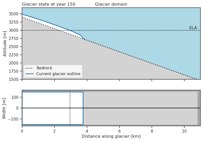
Now we can clearly see the difference between the surface of the glacier and the bedrock. Let’s print the same set of statistics about the glacier as before:
glacier
| Attribute | |
|---|---|
| Id | 1 |
| Type | Glacier |
| Age | 150 |
| Length [m] | 3800.0 |
| Area [km2] | 1.14 |
| Volume [km3] | 0.123785 |
| Max ice thickness [m] | 120.698701 |
| Max ice velocity [m/yr] | 45.91580790745007 |
| AAR [%] | 76.315789 |
| Response time [yrs] | NaN |
| Creep (Glen A) | 2.4e-24 |
| Basal sliding | 0 |
Compare this “numerical glacier” with the “glacier goo” we made in the lab:
How long does it take for the glacier goo to “grow” and flow down the slope? How long does the numerical glacier need?
Below the ELA (3000 m) something happens for the numerical glacier (and for real glaciers too) that did not happen in the glacier goo experiment. What is it?
If we want to calculate changes further in time, we have to set the desired date.
Try editing the cell below to ask the model to run for 500 years instead of 150.
runtime = 150
glacier.progress_to_year(runtime)
/usr/local/pyenv/versions/3.10.12/lib/python3.10/site-packages/oggm_edu/glacier.py:559: UserWarning: Year has to be above the current age of the glacier. It is not possible to de-age the glacier. Geometry will remain the same.
  warnings.warn(msg)
glacier.plot()
glacier
| Attribute | |
|---|---|
| Id | 1 |
| Type | Glacier |
| Age | 150 |
| Length [m] | 3800.0 |
| Area [km2] | 1.14 |
| Volume [km3] | 0.123785 |
| Max ice thickness [m] | 120.698701 |
| Max ice velocity [m/yr] | 45.91580790745007 |
| AAR [%] | 76.315789 |
| Response time [yrs] | NaN |
| Creep (Glen A) | 2.4e-24 |
| Basal sliding | 0 |
Based on this information, do you think you modified the cell correctly?
It is important to note that the model will not go back in time. Once it has run for 500 years, the model will not go back to the 450-year date. It remains at year 500. Try running the cell below. Does the output match what you expected?
glacier.progress_to_year(450)
glacier
| Attribute | |
|---|---|
| Id | 1 |
| Type | Glacier |
| Age | 450 |
| Length [m] | 5700.0 |
| Area [km2] | 1.71 |
| Volume [km3] | 0.187839 |
| Max ice thickness [m] | 122.479449 |
| Max ice velocity [m/yr] | 45.91580790745007 |
| AAR [%] | 52.631579 |
| Response time [yrs] | NaN |
| Creep (Glen A) | 2.4e-24 |
| Basal sliding | 0 |
Accessing the glacier history#
Lucky for us, the Glacier object has also been storing a history of how the glacier has changed over the simulation. We can access that data through the history:
glacier.history
<xarray.Dataset>
Dimensions:           (time: 451)
Coordinates:
  * time              (time) float64 0.0 1.0 2.0 3.0 ... 447.0 448.0 449.0 450.0
    calendar_year     (time) int64 0 1 2 3 4 5 6 ... 444 445 446 447 448 449 450
    calendar_month    (time) int64 1 1 1 1 1 1 1 1 1 1 1 ... 1 1 1 1 1 1 1 1 1 1
    hydro_year        (time) int64 0 1 2 3 4 5 6 ... 444 445 446 447 448 449 450
    hydro_month       (time) int64 4 4 4 4 4 4 4 4 4 4 4 ... 4 4 4 4 4 4 4 4 4 4
Data variables:
    volume_m3         (time) float64 0.0 6.047e+05 ... 1.878e+08 1.878e+08
    volume_bsl_m3     (time) float64 0.0 0.0 0.0 0.0 0.0 ... 0.0 0.0 0.0 0.0 0.0
    volume_bwl_m3     (time) float64 0.0 0.0 0.0 0.0 0.0 ... 0.0 0.0 0.0 0.0 0.0
    area_m2           (time) float64 0.0 6.9e+05 6.9e+05 ... 1.71e+06 1.71e+06
    length_m          (time) float64 0.0 2.3e+03 2.3e+03 ... 5.7e+03 5.7e+03
    calving_m3        (time) float64 0.0 0.0 0.0 0.0 0.0 ... 0.0 0.0 0.0 0.0 0.0
    calving_rate_myr  (time) float64 0.0 0.0 0.0 0.0 0.0 ... 0.0 0.0 0.0 0.0 0.0
Attributes: (12/13)
    description:          OGGM model output
    oggm_version:         1.6.1
    calendar:             365-day no leap
    creation_date:        2023-08-27 22:03:56
    water_level:          0
    glen_a:               2.4e-24
    ...                   ...
    mb_model_class:       MassBalance
    mb_model_hemisphere:  nh
    mb_model_rho:         900.0
    mb_model_orig_ela_h:  3000
    mb_model_ela_h:       3000
mb_model_grad: 4And we can quickly visualise the history of the glacier with the .plot_history() method
glacier.plot_history()
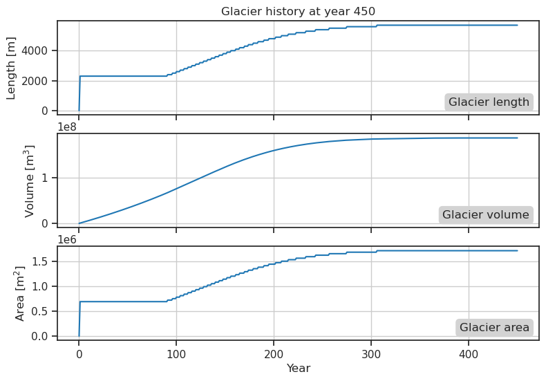
What is going on in this image?
The length of the glacier is a step function in the first year of simulation because, above the equilibrium line altitude (ELA), only accumulation is happening. After that, at first the length of the glacier remains constant. The ice is not very thick, so the portion that reaches below the ELA does not survive the melting that occurs there. But no matter how thick the glacier is, the part above the ELA is always gaining mass. Eventually, there is enough ice to persist below the ELA. We will learn more about ELA in the accumulation and ablation notebook.
Equilibrium state#
After several centuries, the glacier reaches a balance with its climate.
This means that its length and volume will no longer change, as long as all physical parameters and the climate stay roughly constant.
The Glacier object has a method which can progress the glacier to equilibrium .progress_to_equilibrium(). More on this in later notebooks.
Can you identify an equilibrium state in the plots above?
A first experiment#
Ok, we have seen the basics. Now, how about a glacier on a different slope? Glaciers are sometimes very steep, like this one in Nepal.
![]()
Let’s adjust the slope in the model to observe a steeper glacier:
In the following code, can you identify where we tell the model the new slope we are going to use?
What slope did we use for the first experiment? Look for that information at the beginning of the notebook.
# define new slope
new_slope = 20

# create a linear bedrock profile from top to bottom
new_bed = GlacierBed(top=top_elev, bottom=bottom_elev, width=bed_width, slopes=new_slope)

new_glacier = Glacier(bed=new_bed, mass_balance=mb_model)
Comparing glaciers#
We can now introduce the GlacierCollection. This is a utility which can store multiple glaciers and can be used to easily compare and run experiments on multiple glaciers.
# We initialise a collection
collection = GlacierCollection()
# And then add the two glaciers available in this notebook.
collection.add([glacier, new_glacier])
We can get a quick look at the collection by simply calling it:
collection
| Id | Type | Age | Length [m] | Area [km2] | Volume [km3] | Max ice thickness [m] | Max ice velocity [m/yr] | AAR [%] | Response time [yrs] | ... | Basal sliding | Bed type | Top [m] | Bottom [m] | Width(s) [m] | Length [km] | ELA [m] | Original ELA [m] | Temperature bias [C] | Gradient [mm/m/yr] | |
|---|---|---|---|---|---|---|---|---|---|---|---|---|---|---|---|---|---|---|---|---|---|
| Glacier | |||||||||||||||||||||
| 1 | 1 | Glacier | 450 | 5700.0 | 1.71 | 0.187839 | 122.479449 | 45.915808 | 52.631579 | NaN | ... | 0 | Linear bed with a constant width | 3400 | 1500 | 300 | 10.775435 | 3000 | 3000 | 0 | 4 |
| 2 | 2 | Glacier | 0 | 0.0 | 0.00 | 0.000000 | 0.000000 | None | NaN | NaN | ... | 0 | Linear bed with a constant width | 3400 | 1500 | 300 | 5.220207 | 3000 | 3000 | 0 | 4 |
2 rows × 21 columns
Before we compare the glaciers in the collection, let’s make sure to progress them to the same year with the .progress_to_year() method.
collection.progress_to_year(600)
Now let’s compare the glacier we studied first with our new glacier on a different slope. Do you think the new glacier will have more or less ice than the first?
collection.plot_side_by_side(figsize=(10, 5))
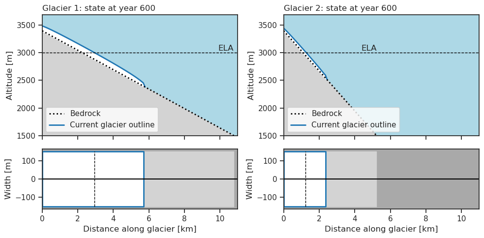
Let’s make sure we understand what is going on:
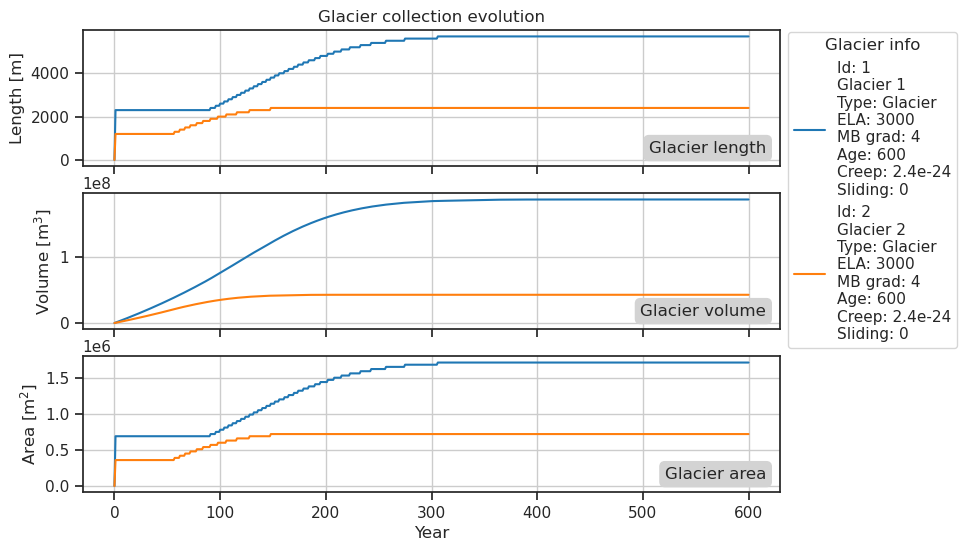
collection.plot_history()
collection
| Id | Type | Age | Length [m] | Area [km2] | Volume [km3] | Max ice thickness [m] | Max ice velocity [m/yr] | AAR [%] | Response time [yrs] | ... | Basal sliding | Bed type | Top [m] | Bottom [m] | Width(s) [m] | Length [km] | ELA [m] | Original ELA [m] | Temperature bias [C] | Gradient [mm/m/yr] | |
|---|---|---|---|---|---|---|---|---|---|---|---|---|---|---|---|---|---|---|---|---|---|
| Glacier | |||||||||||||||||||||
| 1 | 1 | Glacier | 600 | 5700.0 | 1.71 | 0.187843 | 122.479457 | 45.915808 | 52.631579 | NaN | ... | 0 | Linear bed with a constant width | 3400 | 1500 | 300 | 10.775435 | 3000 | 3000 | 0 | 4 |
| 2 | 2 | Glacier | 600 | 2400.0 | 0.72 | 0.042930 | 65.116723 | 34.349697 | 54.166667 | NaN | ... | 0 | Linear bed with a constant width | 3400 | 1500 | 300 | 5.220207 | 3000 | 3000 | 0 | 4 |
2 rows × 21 columns
Explore the characteristics (thickness, length, velocity...). Can you explain the difference between the two glaciers? Click for details
The steeper glacier transports mass from top to bottom faster than the other. As a result, it is overall thinner since the mass gain at the top is the same in both cases (or is it? look at the profiles plot and spot the differences…), but the downward transport means that ice has less time to accumulate before being transported down the ELA and melted away. There is a bit more to the story, but more on this in class!
Activity#
Now, try to change the slope to another value, and run the model again. What do you see?