Ingest gridded products such as ice velocity into OGGM
Contents
Ingest gridded products such as ice velocity into OGGM#
After running our OGGM experiments we often want to compare the model output to other gridded observations or maybe we want to use additional data sets that are not currently in the OGGM shop to calibrate parameters in the model (e.g. Glen A creep parameter, sliding parameter or the calving constant of proportionality). If you are looking on ways or ideas on how to do this, you are in the right tutorial!
In OGGM, a local map projection is defined for each glacier entity in the RGI inventory following the methods described in Maussion and others (2019). The model uses a Transverse Mercator projection centred on the glacier. A lot of data sets, especially those from Polar regions can have a different projections and if we are not careful, we would be making mistakes when we compare them with our model output or when we use such data sets to constrain our model experiments.
NOTE: This code needs OGGM v1.5.3 to run.
First lets import the modules we need:
import xarray as xr
import numpy as np
import matplotlib.pyplot as plt
import salem
from oggm import cfg, utils, workflow, tasks, graphics
cfg.initialize(logging_level='WARNING')
2023-03-07 12:28:46: oggm.cfg: Reading default parameters from the OGGM `params.cfg` configuration file.
2023-03-07 12:28:46: oggm.cfg: Multiprocessing switched OFF according to the parameter file.
2023-03-07 12:28:46: oggm.cfg: Multiprocessing: using all available processors (N=2)
cfg.PATHS['working_dir'] = utils.gettempdir(dirname='OGGM-shop-on-Flowlines', reset=True)
Lets define the glaciers for the run#
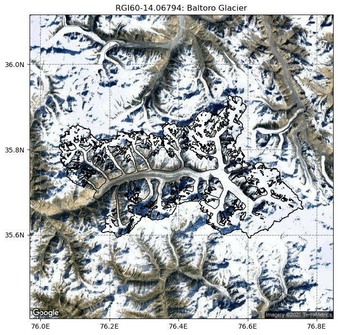
rgi_ids = ['RGI60-14.06794'] # Baltoro
# The RGI version to use
# Size of the map around the glacier.
prepro_border = 80
# Degree of processing level. This is OGGM specific and for the shop 1 is the one you want
from_prepro_level = 3
# URL of the preprocessed gdirs
# we use elevation bands flowlines here
base_url = 'https://cluster.klima.uni-bremen.de/~oggm/gdirs/oggm_v1.4/L3-L5_files/CRU/elev_bands/qc3/pcp2.5/no_match/'

gdirs = workflow.init_glacier_directories(rgi_ids,
                                          from_prepro_level=from_prepro_level,
                                          prepro_base_url=base_url,
                                          prepro_border=prepro_border)
2023-03-07 12:28:46: oggm.workflow: init_glacier_directories from prepro level 3 on 1 glaciers.
2023-03-07 12:28:46: oggm.workflow: Execute entity tasks [gdir_from_prepro] on 1 glaciers
gdir = gdirs[0]
graphics.plot_googlemap(gdir, figsize=(8, 7))
The gridded_data file in the glacier directory#
A lot of the data that the model use and produce for a glacier is stored under the glaciers directories in a NetCDF file called gridded_data:
fpath = gdir.get_filepath('gridded_data')
fpath
'/tmp/OGGM/OGGM-shop-on-Flowlines/per_glacier/RGI60-14/RGI60-14.06/RGI60-14.06794/gridded_data.nc'
with xr.open_dataset(fpath) as ds:
    ds = ds.load()
ds
<xarray.Dataset>
Dimensions: (x: 479, y: 346)
Coordinates:
* x (x) float32 -4.764e+04 -4.744e+04 ... 4.776e+04 4.796e+04
* y (y) float32 3.992e+06 3.992e+06 ... 3.923e+06 3.923e+06
Data variables:
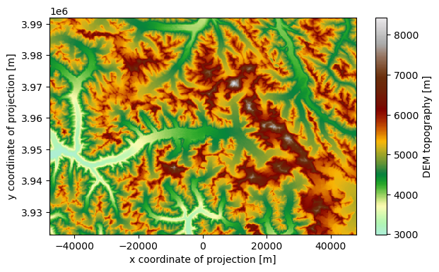
topo (y, x) float32 5.128e+03 4.999e+03 ... 5.291e+03 5.299e+03
topo_smoothed (y, x) float32 5.113e+03 5.019e+03 ... 5.291e+03 5.295e+03
topo_valid_mask (y, x) int8 1 1 1 1 1 1 1 1 1 1 1 ... 1 1 1 1 1 1 1 1 1 1 1
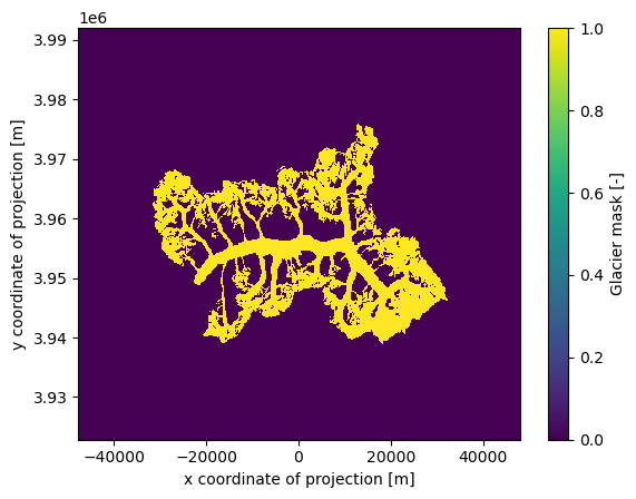
glacier_mask (y, x) int8 0 0 0 0 0 0 0 0 0 0 0 ... 0 0 0 0 0 0 0 0 0 0 0
glacier_ext (y, x) int8 0 0 0 0 0 0 0 0 0 0 0 ... 0 0 0 0 0 0 0 0 0 0 0
Attributes:
author: OGGM
author_info: Open Global Glacier Model
pyproj_srs: +proj=tmerc +lat_0=0 +lon_0=76.4047 +k=0.9996 +x_0=0 +y_0...
max_h_dem: 8437.0
min_h_dem: 2996.0
max_h_glacier: 8437.0
min_h_glacier: 3397.0cmap=salem.get_cmap('topo')
ds.topo.plot(figsize=(7, 4), cmap=cmap);
ds.glacier_mask.plot();
Add data from OGGM-Shop: bed topography data#
Additionally to the data produced by the model, the OGGM-Shop counts with routines that will automatically download and reproject other useful data sets into the glacier projection (For more information also check out this notebook). This data will be stored under the file described above.
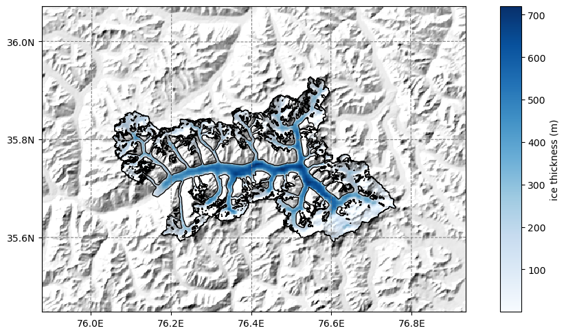
OGGM can now download data from the Farinotti et al., (2019) consensus estimate and reproject it to the glacier directories map:
from oggm.shop import bedtopo
workflow.execute_entity_task(bedtopo.add_consensus_thickness, gdirs);
2023-03-07 12:28:59: oggm.workflow: Execute entity tasks [add_consensus_thickness] on 1 glaciers
with xr.open_dataset(gdir.get_filepath('gridded_data')) as ds:
    ds = ds.load()
the cell below might take a while… be patient
# plot the salem map background, make countries in grey
smap = ds.salem.get_map(countries=False)
smap.set_shapefile(gdir.read_shapefile('outlines'))
smap.set_topography(ds.topo.data);
f, ax = plt.subplots(figsize=(9, 9))
smap.set_data(ds.consensus_ice_thickness)
smap.set_cmap('Blues')
smap.plot(ax=ax)
smap.append_colorbar(ax=ax, label='ice thickness (m)');
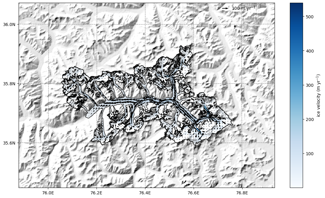
OGGM-Shop: ITS-live#
This is an example on how to extract velocity fields from the ITS_live Regional Glacier and Ice Sheet Surface Velocities Mosaic (Gardner, A. et al 2019) at 120 m resolution and reproject this data to the OGGM-glacier grid. This only works where ITS-live data is available! (not in the Alps).
The data source used is https://its-live.jpl.nasa.gov/#data.
Currently the only data downloaded is the 120m composite for both (u, v) and their uncertainty. The composite is computed from the 1985 to 2018 average. If you want more velocity products, feel free to open a new topic on the OGGM issue tracker!
this will download severals large dataset (2~800MB) depending on your connection might take a bit …
from oggm.shop import its_live
workflow.execute_entity_task(its_live.velocity_to_gdir, gdirs);
2023-03-07 12:29:11: oggm.workflow: Execute entity tasks [velocity_to_gdir] on 1 glaciers
By applying the entity task its_live.velocity_to_gdir() OGGM downloads and reprojects the ITS_live files to a given glacier map.
The velocity components (vx, vy) are added to the gridded_data nc file.
According to the ITS_LIVE documentation velocities are given in ground units (i.e. absolute velocities). We then use bilinear interpolation to reproject the velocities to the local glacier map by re-projecting the vector distances (For more details feel free to checl out the code).
By specifying add_error=True on its_live.velocity_to_gdir(gdir, add_error=True), we also reproject and scale the error for each component (evx, evy).
Now we can read in all the gridded data that comes with OGGM, including the ITS_Live velocity components.
with xr.open_dataset(gdir.get_filepath('gridded_data')) as ds:
    ds = ds.load()
ds
<xarray.Dataset>
Dimensions:                  (x: 479, y: 346)
Coordinates:
  * x                        (x) float32 -4.764e+04 -4.744e+04 ... 4.796e+04
  * y                        (y) float32 3.992e+06 3.992e+06 ... 3.923e+06
Data variables:
    topo                     (y, x) float32 5.128e+03 4.999e+03 ... 5.299e+03
    topo_smoothed            (y, x) float32 5.113e+03 5.019e+03 ... 5.295e+03
    topo_valid_mask          (y, x) int8 1 1 1 1 1 1 1 1 1 ... 1 1 1 1 1 1 1 1 1
    glacier_mask             (y, x) int8 0 0 0 0 0 0 0 0 0 ... 0 0 0 0 0 0 0 0 0
    glacier_ext              (y, x) int8 0 0 0 0 0 0 0 0 0 ... 0 0 0 0 0 0 0 0 0
    consensus_ice_thickness  (y, x) float32 nan nan nan nan ... nan nan nan nan
    obs_icevel_x             (y, x) float32 -0.3372 -0.3311 ... -16.64 -19.13
    obs_icevel_y             (y, x) float32 1.797 5.185 8.147 ... 33.85 38.78
Attributes:
    author:         OGGM
    author_info:    Open Global Glacier Model
    pyproj_srs:     +proj=tmerc +lat_0=0 +lon_0=76.4047 +k=0.9996 +x_0=0 +y_0...
    max_h_dem:      8437.0
    min_h_dem:      2996.0
    max_h_glacier:  8437.0
min_h_glacier: 3397.0# plot the salem map background, make countries in grey
smap = ds.salem.get_map(countries=False)
smap.set_shapefile(gdir.read_shapefile('outlines'))
smap.set_topography(ds.topo.data);
# get the velocity data
u = ds.obs_icevel_x.where(ds.glacier_mask == 1)
v = ds.obs_icevel_y.where(ds.glacier_mask == 1)
ws = (u**2 + v**2)**0.5
The ds.glacier_mask == 1 command will remove the data outside of the glacier outline.
# get the axes ready
f, ax = plt.subplots(figsize=(12, 12))

# Quiver only every 3rd grid point
us = u[1::5, 1::5]
vs = v[1::5, 1::5]

smap.set_data(ws)
smap.set_cmap('Blues')
smap.plot(ax=ax)
smap.append_colorbar(ax=ax, label = 'ice velocity (m yr$^{-1}$)')

# transform their coordinates to the map reference system and plot the arrows
xx, yy = smap.grid.transform(us.x.values, us.y.values, crs=gdir.grid.proj)
xx, yy = np.meshgrid(xx, yy)
qu = ax.quiver(xx, yy, us.values, vs.values)
qk = ax.quiverkey(qu, 0.82, 0.97, 100, '100 m yr$^{-1}$',
                   labelpos='E', coordinates='axes')
Bin the data in gridded_data into OGGM elevation bands#
Now that we have added new data to the gridded_data file, we can bin the data sets into the same elevation bands as OGGM by recomputing the elevation bands flowlines:
tasks.elevation_band_flowline(gdir,
                              bin_variables=['consensus_ice_thickness', 'obs_icevel_x', 'obs_icevel_y'],
                              preserve_totals=[True, False, False]  # I"m actually not sure if preserving totals is meaningful with velocities - likely not
                              )
This created a csv in the glacier directory folder with the data binned to it:
import pandas as pd
df = pd.read_csv(gdir.get_filepath('elevation_band_flowline'), index_col=0)
df
| area | mean_elevation | slope | consensus_ice_thickness | obs_icevel_x | obs_icevel_y | bin_elevation | dx | width | |
|---|---|---|---|---|---|---|---|---|---|
| dis_along_flowline | |||||||||
| 60.172585 | 40000.0 | 8345.080078 | 0.244304 | 18.147763 | -0.191088 | 0.212503 | 8355.0 | 120.345169 | 332.377280 |
| 140.404661 | 80000.0 | 8235.238281 | 0.642076 | 13.891147 | -0.119776 | 0.298178 | 8235.0 | 40.118984 | 1994.068447 |
| 173.940860 | 40000.0 | 8197.490234 | 0.838840 | 21.082249 | -0.173281 | 0.277646 | 8205.0 | 26.953414 | 1484.042070 |
| 202.717642 | 40000.0 | 8150.462891 | 0.775495 | 25.654437 | 0.060681 | 0.333409 | 8145.0 | 30.600150 | 1307.183150 |
| 236.363889 | 40000.0 | 8075.439941 | 0.685386 | 14.702222 | 0.089171 | 0.122661 | 8085.0 | 36.692346 | 1090.145619 |
| ... | ... | ... | ... | ... | ... | ... | ... | ... | ... |
| 42308.885990 | 760000.0 | 3525.279541 | 0.104131 | 139.481158 | -4.474717 | -2.795007 | 3525.0 | 287.057248 | 2647.555512 |
| 42583.856935 | 400000.0 | 3495.227295 | 0.113627 | 101.916241 | -3.964900 | -2.077398 | 3495.0 | 262.884641 | 1521.579952 |
| 42814.941987 | 200000.0 | 3472.789551 | 0.149416 | 98.673038 | -4.508717 | -1.815381 | 3465.0 | 199.285463 | 1003.585494 |
| 43010.329233 | 200000.0 | 3441.432373 | 0.155404 | 59.133279 | -2.572173 | -1.226399 | 3435.0 | 191.489029 | 1044.446259 |
| 43224.984756 | 120000.0 | 3407.177490 | 0.125482 | 32.996786 | -0.836834 | -0.399884 | 3405.0 | 237.822018 | 504.579018 |
157 rows × 9 columns
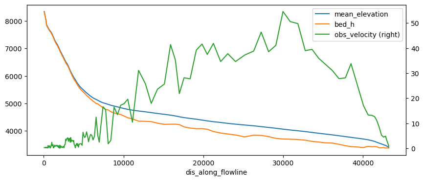
df['obs_velocity'] = (df['obs_icevel_x']**2 + df['obs_icevel_y']**2)**0.5
df['bed_h'] = df['mean_elevation'] - df['consensus_ice_thickness']
df[['mean_elevation', 'bed_h', 'obs_velocity']].plot(figsize=(10, 4), secondary_y='obs_velocity');
The problem with this file is that it does not have a regular spacing. The numerical model needs regular spacing, which is why OGGM does this:
# This takes the csv file and prepares new 'inversion_flowlines.pkl' and created a new csv file with regular spacing
tasks.fixed_dx_elevation_band_flowline(gdir,
                                       bin_variables=['consensus_ice_thickness', 'obs_icevel_x', 'obs_icevel_y'],
                                       preserve_totals=[True, False, False]
                                      )
df_regular = pd.read_csv(gdir.get_filepath('elevation_band_flowline', filesuffix='_fixed_dx'), index_col=0)
df_regular
| widths_m | area_m2 | consensus_ice_thickness | obs_icevel_x | obs_icevel_y | |
|---|---|---|---|---|---|
| dis_along_flowline | |||||
| 200.0 | 1350.508131 | 5.402033e+05 | 24.852592 | 0.038586 | 0.328143 |
| 600.0 | 1557.488984 | 6.229956e+05 | 12.058255 | -0.115721 | 0.288789 |
| 1000.0 | 7529.527187 | 3.011811e+06 | 32.532095 | 2.174206 | 0.080531 |
| 1400.0 | 15906.311989 | 6.362525e+06 | 29.213418 | 0.595236 | 0.310646 |
| 1800.0 | 35987.148540 | 1.439486e+07 | 42.631021 | 0.415668 | 0.740916 |
| ... | ... | ... | ... | ... | ... |
| 41400.0 | 2128.789125 | 8.515156e+05 | 188.005470 | -5.837341 | -11.296937 |
| 41800.0 | 1795.906259 | 7.183625e+05 | 163.145085 | -7.081799 | -7.600463 |
| 42200.0 | 2387.409586 | 9.549638e+05 | 148.023098 | -5.238625 | -3.783761 |
| 42600.0 | 1515.264571 | 6.061058e+05 | 100.197741 | -4.002890 | -2.059094 |
| 43000.0 | 1063.245975 | 4.252984e+05 | 60.325326 | -2.674549 | -1.257536 |
108 rows × 5 columns
The other variables have disappeared for saving space, but I think it would be nicer to have them here as well. We can grab them from the inversion flowlines (this could be better handled in OGGM):
fl = gdir.read_pickle('inversion_flowlines')[0]
df_regular['mean_elevation'] = fl.surface_h
df_regular['obs_velocity'] = (df_regular['obs_icevel_x']**2 + df_regular['obs_icevel_y']**2)**0.5
df_regular['consensus_bed_h'] = df_regular['mean_elevation'] - df_regular['consensus_ice_thickness']
df_regular[['mean_elevation', 'consensus_bed_h', 'obs_velocity']].plot(figsize=(10, 4), secondary_y='obs_velocity');
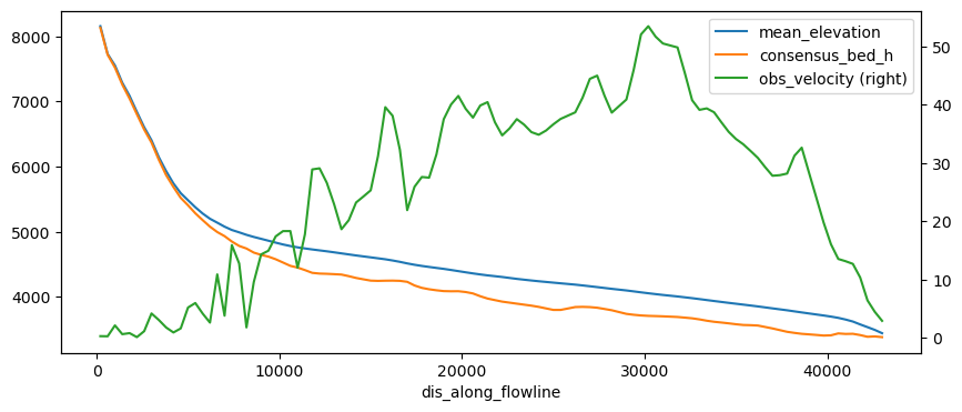
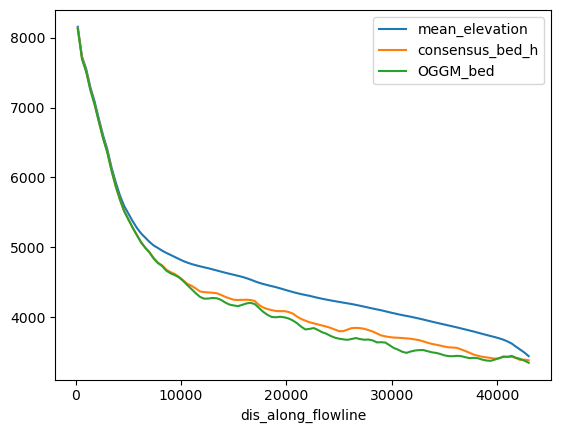
OK so more or less the same but this time on a regular grid. Note that these now have the same length as the OGGM inversion flowlines, i.e. one can do stuff such as comparing what OGGM has done for the inversion:
inv = gdir.read_pickle('inversion_output')[0]
df_regular['OGGM_bed'] = df_regular['mean_elevation'] - inv['thick']
df_regular[['mean_elevation', 'consensus_bed_h', 'OGGM_bed']].plot();
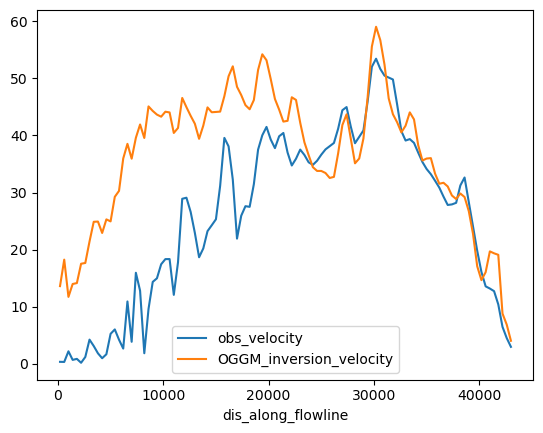
Compare velocities: at inversion#
OGGM already inverted the ice thickness based on some optimisation such as matching the regional totals. Which parameters did we use?
d = gdir.get_diagnostics()
d
{'dem_source': 'NASADEM',
 'flowline_type': 'elevation_band',
 'inversion_glen_a': 2.2535112971797524e-24,
 'inversion_fs': 0}
# OK set them so that we are consistent
cfg.PARAMS['inversion_glen_a'] = d['inversion_glen_a']
cfg.PARAMS['inversion_fs'] = d['inversion_fs']
2023-03-07 12:29:30: oggm.cfg: PARAMS['inversion_glen_a'] changed from `2.4e-24` to `2.2535112971797524e-24`.
# Since we overwrote the inversion flowlines we have to do stuff again
utils.apply_test_ref_tstars()
tasks.local_t_star(gdir)
tasks.mu_star_calibration(gdir)
tasks.prepare_for_inversion(gdir, add_debug_var=True)
tasks.mass_conservation_inversion(gdir)
tasks.compute_velocities(gdir)
inv = gdir.read_pickle('inversion_output')[0]
df_regular['OGGM_inversion_velocity'] = inv['u_surface']
df_regular[['obs_velocity', 'OGGM_inversion_velocity']].plot();
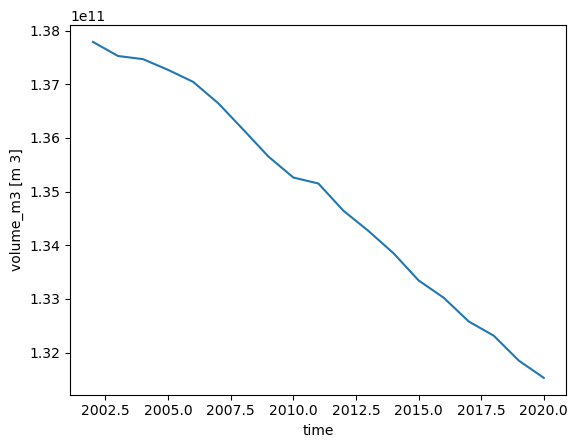
Velocities during the run#
Inversion velocities are for a glacier at equilibrium - this is not always meaningful. Lets do a run and store the velocities with time:
cfg.PARAMS['store_fl_diagnostics'] = True

# if you start to look into velocities, you will see that OGGM is quite large
# regarding numerical stabilities - here is a better default (yet not perfect)
cfg.PARAMS['cfl_number'] = 0.01
2023-03-07 12:29:30: oggm.cfg: PARAMS['store_fl_diagnostics'] changed from `False` to `True`.
2023-03-07 12:29:30: oggm.cfg: PARAMS['cfl_number'] changed from `0.02` to `0.01`.
tasks.run_from_climate_data(gdir);
/usr/local/pyenv/versions/3.10.10/lib/python3.10/site-packages/oggm/utils/_workflow.py:2939: UserWarning: Unpickling a shapely <2.0 geometry object. Please save the pickle again; shapely 2.1 will not have this compatibility.
  out = pickle.load(f)
with xr.open_dataset(gdir.get_filepath('model_diagnostics')) as ds_diag:
    ds_diag = ds_diag.load()
ds_diag.volume_m3.plot();
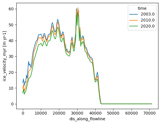
with xr.open_dataset(gdir.get_filepath('fl_diagnostics'), group='fl_0') as ds_fl:
    ds_fl = ds_fl.load()
ds_fl
<xarray.Dataset>
Dimensions:             (dis_along_flowline: 179, time: 19)
Coordinates:
  * dis_along_flowline  (dis_along_flowline) float64 0.0 400.0 ... 7.12e+04
  * time                (time) float64 2.002e+03 2.003e+03 ... 2.02e+03
Data variables:
    point_lons          (dis_along_flowline) float64 75.88 75.88 ... 76.66 76.67
    point_lats          (dis_along_flowline) float64 36.07 36.07 ... 36.07 36.07
    bed_h               (dis_along_flowline) float64 8.129e+03 ... 3.007e+03
    volume_m3           (time, dis_along_flowline) float64 1.377e+07 ... 0.0
    volume_bsl_m3       (time, dis_along_flowline) float64 0.0 0.0 ... 0.0 0.0
    volume_bwl_m3       (time, dis_along_flowline) float64 0.0 0.0 ... 0.0 0.0
    area_m2             (time, dis_along_flowline) float64 5.402e+05 ... 0.0
    thickness_m         (time, dis_along_flowline) float64 25.99 36.33 ... 0.0
    ice_velocity_myr    (time, dis_along_flowline) float64 nan nan ... 0.0 0.0
    calving_bucket_m3   (time) float64 0.0 0.0 0.0 0.0 0.0 ... 0.0 0.0 0.0 0.0
Attributes:
    class:                MixedBedFlowline
    map_dx:               200.0
    dx:                   2.0
    description:          OGGM model output
    oggm_version:         1.5.3
    calendar:             365-day no leap
    creation_date:        2023-03-07 12:29:30
    water_level:          0
    glen_a:               2.2535112971797524e-24
    fs:                   0
    mb_model_class:       MultipleFlowlineMassBalance
mb_model_hemisphere: nhds_fl.sel(time=[2003, 2010, 2020]).ice_velocity_myr.plot(hue='time');
# The OGGM model flowlines also have the downstream lines
df_regular['OGGM_velocity_run_begin'] = ds_fl.sel(time=2003).ice_velocity_myr.data[:len(df_regular)]
df_regular['OGGM_velocity_run_end'] = ds_fl.sel(time=2020).ice_velocity_myr.data[:len(df_regular)]
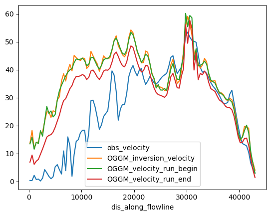
df_regular[['obs_velocity', 'OGGM_inversion_velocity', 'OGGM_velocity_run_begin', 'OGGM_velocity_run_end']].plot();