Dynamic spinup and dynamic melt_f calibration for past simulations#
New in version 1.5.3 resp. version 1.6.0!
One of the issues glacier modellers facing is that the past state of glaciers is unknown. On the other side, more global datasets of past observations get available (e.g. geodetic mass balance), which can help constrain the recent past evolution.
Reconstructing the past states of glaciers on a century timescale turns out to be a really difficult task, and OGGM team member Julia Eis spent her entire PhD thesis doing just that (see this paper for the theory and this one for the application).
However, running simulations in the recent past can be quite useful for model validation. Also, more direct observations are available of glacier states of the recent past for constriction (e.g. area, geodetic mass balance). Further, a dynamical initialisation can release strong assumptions in the OGGM default settings: first that glaciers are in dynamical equilibrium at the glacier outline date (an assumption required for the ice thickness inversion) and second that the mass balance melt factor parameter (melt_f) is calibrated towards a geodetic mass balance ignoring a dynamically changing glacier geometry.
In recent PRs (GH1342, GH1232, GH1361 and GH1425) we have released two new run tasks in OGGM which help with this issues:
The
run_dynamic_spinuptask, by default, aims to find a glacier state before the RGI-date (~10-30 years back) from which the glacier evolves to match the area given by the RGI-outline. Alternatively, it is also possible to use this task to match an observed volume.The
run_dynamic_melt_f_calibrationtask iteratively searches for a melt_f to match the observed geodetic mass balance taking a dynamically changing glacier geometry into account.
And of course, we want to match both things in the same past model run. Therefore by default in each iteration of run_dynamic_melt_f_calibration the run_dynamic_spinup function is included. A more in-depth explanation of the two tasks is provided in the next two chapters, which are followed by an example and a comparison of the different spinup options.
High-level explanation of run_dynamic_spinup:#
The dynamic spinup iteratively tries to find an initial glacier state in the past (t_start) that matches the area or the volume at the glacier outline date (t_end) under the historical climate forcing. To create changing initial glacier states, a constant mass balance is used (mb_spinup) together with a changing temperature bias. This mass balance defines an average mass balance between t_start and t_end. Afterwards, for the actual run, the method uses the OGGM default mass balance model (mb_historical). One iteration of the dynamic spinup looks like this:
Apply a temperature bias to mb_spinup.
Start with the glacier geometry after the ice thickness inversion and let the model evolve using mb_spinup for the same amount of time as the following historical run (= t_end - t_start).
The resulting glacier geometry is defined as the initial glacier state at t_start.
Now, let the glacier evolve using mb_historical from t_start until t_end
Get the model area or volume of the glacier at t_end.
Compare the model value to the reference value we want to meet.
If the difference is inside a given precision, stop the procedure and save the glacier evolution of this run.
If the difference is outside a given precision, change the temperature bias for mb_spinup and start over again (how the next guess is found is descript here).
With OGGM version 1.6.1 it is now also possible to provide a custom target year target_yr with target value target_value to match. This could be useful if you have more data available than on a global scale (e.g. an extra outline at a later date than the RGI).
Two main problems why the dynamic spinup could not work:#
The resulting glacier is too large, even when we start from a completely ice-free initial glacier state. Or the resulting glacier is too small and the algorithm tries to let the glacier grow outside the domain boundaries. The second problem could be met with a larger domain boundary (if available and enough memory resources are available). But for the first problem, no such solution is possible. To still try to cope with these two issues the dynamic spinup function tries to shorten the dynamic spinup period two times. The idea is with a shorter evolution time the glacier has less amount of time to grow/shrink and maybe do not encounter one of the two extremes. The minimum length of the spinup can be defined with min_spinup_period (default 10 years). If nothing helps and there is still an error (and if ignore_errors = True) the glacier geometry without a dynamic spinup is saved (= the glacier geometry after the ice thickness inversion).
If the period was shortened it is possible to add a fixed geometry spinup at the beginning (see example below). With this you can make sure that all glaciers start at the defined starting year.
¡Careful! This method is still a bit experimental. A few things to remember when using it:#
because of how the method works, glacier area and volume are not strictly the same at the glacier inventory date as after the inversion. We have checked that the errors are random: if you simulate many glaciers this should be fine (global plots on this point will follow soon).
because of the non-unique solutions to this optimization problem, the estimated past states become increasingly uncertain the further back in time we go. We recommend a spinup of about 10-30 years.
High-level explanation of run_dynamic_melt_f_calibration :#
This task iteratively searches for a melt_f to match a given geodetic mass balance incorporating a dynamic model run. But changing melt_f means we need to rerun all model setup steps which incorporate the mass-balance, to have one consistent model initialisation chain. In particular, we need to conduct the bed inversion again (the mass-balance is used in the flux calculation, see here). Therefore one default iteration of the dynamic melt_f calibration looks like this:
define a new melt_f in the glacier directory
conduct an inversion which calibrates to the consensus volume, still assuming dynamic equilibrium. (a little tricky: by default, before we start with the dynamic melt_f calibration the first inversion with calibration on a regional scale was already carried out -> the individual glaciers do not match the consensus volume exactly, but when adding all glaciers of one region the consensus volume is matched. Therefore during this task, the individual glacier is again matched to the volume of the regional assessment and not on an individual basis.)
conduct a dynamic spinup to match the RGI area and let the model evolve up to the end of the geodetic mass balance period
calculate the modelled geodetic mass balance
calculate the difference between modelled value and observation
if the difference is inside the observation uncertainty stop and save the model run (indicated in diagnostics with
used_spinup_option = dynamic melt_f calibration (full success))if the difference is larger, define a new melt_f and start over again (how the next guess is found is described here)
If the iterative search is not successful and ignore_errors = True there are several possible outcomes:
First, it is checked if there were some successful runs which improved the mismatch. If so, the best run is saved and it is indicated in the diagnostics with
used_spinup_option = dynamic melt_f calibration (part success)If only the first guess worked this run is saved and indicated in the diagnostics with
used_spinup_option = dynamic spinup onlyAnd if everything failed a fixed geometry spinup is conducted and indicated in the diagnostics with
used_spinup_option = fixed geometry spinup
If for whatever reason one wants to conduct the dynamic melt_f calibration without an inversion or does not want to include a dynamic spinup, reach out to us as there are already options included for this.
The minimization algorithm:#
To start, a first guess of the control variable (temperature bias or melt_f) is used and evaluated. If by chance, the mismatch between model and observation is close enough, the algorithm stops already. Otherwise, the second guess depends on the calculated first guess mismatch. For example, if the first resulting area is smaller (larger) than the searched one, the second temperature bias will be colder (warmer). Because a colder (warmer) temperature leads to a larger (smaller) initial glacier state at t_start. If the second guess is still unsuccessful, for all consecutive guesses the previous value pairs (control variable, mismatch) are used to determine the next guess. For this, a stepwise linear function is fitted to these pairs and afterwards, the mismatch is set to 0 to get the following guess (this method is similar to the one described in Zekollari et al. 2019 Appendix A). Moreover, a maximum step length between two guesses is defined as too large step-sizes could easily lead to failing model runs (e.g. see here). Further, the algorithm was adapted independently inside run_dynamic_spinup and run_dynamic_melt_f_calibration to cope with failing model runs individually. Note that this minimization algorithm only works if the underlying relationship between the control variable and the mismatch is strictly monotone.
If someone is interested in how this algorithm works in more detail, here is a conceptual code snippet:
Show code cell source
import numpy as np
from scipy import interpolate

def minimisation_algorithm(
        fct_to_minimise,  # the function which should be minimised
        first_guess,  # the first guess of the control variable
        get_second_guess,  # function which gives the second guess depending on
                           # the first mismatch
        precision_to_match,  # we want to be smaller with the mismatch than this
        maxiter,  # how many search iteration should be performed
        ):

    control_guesses = []
    mismatch = []

    # returns also the new control if some error management was going on inside
    # fct_to_minimise, not necessary
    new_mismatch, new_control = fct_to_minimise(first_guess)
    control_guesses.append(new_control)
    mismatch.append(new_mismatch)

    # check if we can stop already
    if abs(mismatch[-1]) < precision_to_match:
            return control_guesses, mismatch

    # how to get the second guess must also be defined by the user
    second_guess = get_second_guess(mismatch[-1])
    new_mismatch, new_control = fct_to_minimise(second_guess)
    control_guesses.append(new_control)
    mismatch.append(new_mismatch)
    if abs(mismatch[-1]) < precision_to_match:
        return control_guesses, mismatch

    # now we start with the partial linear fitting
    while len(control_guesses) < maxiter:
        # sort the (mismatch, control_pairs) from small to large
        sort_index = np.argsort(np.array(mismatch))
        # actual linear fitting
        tck = interpolate.splrep(np.array(mismatch)[sort_index],
                                 np.array(control_guesses)[sort_index],
                                 k=1)  # degree of the fitting, 1 is linear
        # if there are NaNs in the fitting parameters it is an indication that
        # probably the strictly monotone relation is not holding, but also
        # other problems possible (e.g. to close guesses)
        if np.isnan(tck[1]).any():
            # here is the place where you can do further problem dependent
            # error management or just raise an error
            raise RuntimeError('Somthing went wrong during the linear fitting!')

        # evaluate the linear fit where mismatch = 0 to get the next guess
        next_control_guess = float(interpolate.splev(0, tck))

        new_mismatch, new_control = fct_to_minimise(next_control_guess)
        control_guesses.append(new_control)
        mismatch.append(new_mismatch)
        if abs(mismatch[-1]) < precision_to_match:
            return control_guesses, mismatch

    # If we end here it was not possible to find a satisfying mismatch after maxiter(ations)
    raise RuntimeError('Could not find small enough mismatch after the'
                       'maximum iterations!')
Start with glacier example#
import matplotlib.pyplot as plt
import xarray as xr
import numpy as np
import pandas as pd
import seaborn as sns
# Make pretty plots
sns.set_style('ticks')
sns.set_context('notebook')
from oggm import cfg, utils, workflow, tasks, graphics
cfg.initialize(logging_level='WARNING')
cfg.PATHS['working_dir'] = utils.gettempdir(dirname='OGGM_dynamic_spinup', reset=True)
2023-08-27 23:32:21: oggm.cfg: Reading default parameters from the OGGM `params.cfg` configuration file.
2023-08-27 23:32:21: oggm.cfg: Multiprocessing switched OFF according to the parameter file.
2023-08-27 23:32:21: oggm.cfg: Multiprocessing: using all available processors (N=2)
Define the glaciers we will play with#
# Hintereisferner and a 'bad' glacier in terms of the dynamic spinup
rgi_ids = ['RGI60-11.00897', 'RGI60-11.00275']
Preparing the glacier data#
This can take up to a few minutes on the first call because of the download of the required data:
# We use a recent gdir setting, calibated on a glacier per glacier basis
base_url = ('https://cluster.klima.uni-bremen.de/~oggm/gdirs/oggm_v1.6/'
            'L3-L5_files/2023.3/elev_bands/W5E5/')
# We use a relatively large border value to allow the glacier to grow during spinup
gdirs = workflow.init_glacier_directories(rgi_ids, from_prepro_level=3, prepro_border=160, prepro_base_url=base_url)
2023-08-27 23:32:23: oggm.workflow: init_glacier_directories from prepro level 3 on 2 glaciers.
2023-08-27 23:32:23: oggm.workflow: Execute entity tasks [gdir_from_prepro] on 2 glaciers
Start by comparing three different spinups#
# For the following experiments we only use Khumbu
gdir = gdirs[0]
# We will "reconstruct" a possible glacier evolution from this year onwards
spinup_start_yr = 1979

# here we save the original melt_f for later
melt_f_original = gdir.read_json('mb_calib')['melt_f']

# and save some reference values we can compare to later
area_reference = gdir.rgi_area_m2  # RGI area
volume_reference = tasks.get_inversion_volume(gdir)  # volume after regional calibration to consensus
ref_period = cfg.PARAMS['geodetic_mb_period']  # get the reference period we want to use, 2000 to 2020
df_ref_dmdtda = utils.get_geodetic_mb_dataframe().loc[gdir.rgi_id]  # get the data from Hugonnet 2021
df_ref_dmdtda = df_ref_dmdtda.loc[df_ref_dmdtda['period'] == ref_period]  # only select the desired period
dmdtda_reference = df_ref_dmdtda['dmdtda'].values[0] * 1000  # get the reference dmdtda and convert into kg m-2 yr-1
dmdtda_reference_error = df_ref_dmdtda['err_dmdtda'].values[0] * 1000  # corresponding uncertainty
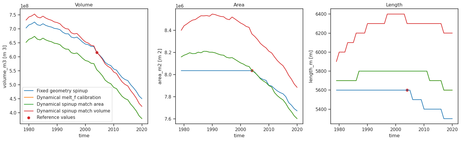
Let’s start by comparing the fixed_geometry_spinup, the run_dynamic_spinup and the run_dynamic_melt_f_calibration (which contains a dynamic spinup) options.
# ---- First do the fixed geometry spinup ----
tasks.run_from_climate_data(gdir,
                            fixed_geometry_spinup_yr=spinup_start_yr,  # Start the run at the RGI date but retro-actively correct the data with fixed geometry
                            output_filesuffix='_hist_fixed_geom',  # where to write the output
                            );
# Read the output
with xr.open_dataset(gdir.get_filepath('model_diagnostics', filesuffix='_hist_fixed_geom')) as ds:
    ds_hist = ds.load()

# ---- Second the dynamic spinup alone, matching area ----
tasks.run_dynamic_spinup(gdir,
                         spinup_start_yr=spinup_start_yr,  # When to start the spinup
                         minimise_for='area',  # what target to match at the RGI date
                         output_filesuffix='_spinup_dynamic_area',  # Where to write the output
                         ye=2020,  # When the simulation should stop
                         );
# Read the output
with xr.open_dataset(gdir.get_filepath('model_diagnostics', filesuffix='_spinup_dynamic_area')) as ds:
    ds_dynamic_spinup_area = ds.load()

# ---- Third the dynamic spinup alone, matching volume ----
tasks.run_dynamic_spinup(gdir,
                         spinup_start_yr=spinup_start_yr,  # When to start the spinup
                         minimise_for='volume',  # what target to match at the RGI date
                         output_filesuffix='_spinup_dynamic_volume',  # Where to write the output
                         ye=2020,  # When the simulation should stop
                         );
# Read the output
with xr.open_dataset(gdir.get_filepath('model_diagnostics', filesuffix='_spinup_dynamic_volume')) as ds:
    ds_dynamic_spinup_volume = ds.load()

# ---- Fourth the dynamic melt_f calibration (includes a dynamic spinup matching area) ----
tasks.run_dynamic_melt_f_calibration(gdir,
                                     ys=spinup_start_yr,  # When to start the spinup
                                     ye=2020,  # When the simulation should stop
                                     output_filesuffix='_dynamic_melt_f',  # Where to write the output
                                    );

with xr.open_dataset(gdir.get_filepath('model_diagnostics', filesuffix='_dynamic_melt_f')) as ds:
    ds_dynamic_melt_f = ds.load()
# Now make a plot for comparision
y0 = gdir.rgi_date + 1

f, (ax1, ax2, ax3) = plt.subplots(1, 3, figsize=(16, 5))

ds_hist.volume_m3.plot(ax=ax1, label='Fixed geometry spinup');
ds_dynamic_melt_f.volume_m3.plot(ax=ax1, label='Dynamical melt_f calibration');
ds_dynamic_spinup_area.volume_m3.plot(ax=ax1, label='Dynamical spinup match area');
ds_dynamic_spinup_volume.volume_m3.plot(ax=ax1, label='Dynamical spinup match volume');
ax1.set_title('Volume');
ax1.scatter(y0, volume_reference, c='C3', label='Reference values');
ax1.legend();

ds_hist.area_m2.plot(ax=ax2);
ds_dynamic_melt_f.area_m2.plot(ax=ax2);
ds_dynamic_spinup_area.area_m2.plot(ax=ax2);
ds_dynamic_spinup_volume.area_m2.plot(ax=ax2);
ax2.set_title('Area');
ax2.scatter(y0, area_reference, c='C3')

ds_hist.length_m.plot(ax=ax3);
ds_dynamic_melt_f.length_m.plot(ax=ax3);
ds_dynamic_spinup_area.length_m.plot(ax=ax3);
ds_dynamic_spinup_volume.length_m.plot(ax=ax3);
ax3.set_title('Length');
ax3.scatter(y0, ds_hist.sel(time=y0).length_m, c='C3')

plt.tight_layout()
plt.show();

# and print out the modeled geodetic mass balances for comparision
def get_dmdtda(ds):
    yr0_ref_mb, yr1_ref_mb = ref_period.split('_')
    yr0_ref_mb = int(yr0_ref_mb.split('-')[0])
    yr1_ref_mb = int(yr1_ref_mb.split('-')[0])

    return ((ds.volume_m3.loc[yr1_ref_mb].values -
             ds.volume_m3.loc[yr0_ref_mb].values) /
            gdir.rgi_area_m2 /
            (yr1_ref_mb - yr0_ref_mb) *
            cfg.PARAMS['ice_density'])

print(f'Reference dmdtda 2000 to 2020 (Hugonnet 2021):     {dmdtda_reference:.2f} +/- {dmdtda_reference_error:6.2f} kg m-2 yr-1')
print(f'Fixed geometry spinup dmdtda 2000 to 2020:         {get_dmdtda(ds_hist):.2f}            kg m-2 yr-1')
print(f'Dynamical spinup match area dmdtda 2000 to 2020:   {get_dmdtda(ds_dynamic_spinup_area):.2f}            kg m-2 yr-1')
print(f'Dynamical spinup match volume dmdtda 2000 to 2020: {get_dmdtda(ds_dynamic_spinup_volume):.2f}            kg m-2 yr-1')
print(f'Dynamical melt_f calibration dmdtda 2000 to 2020:  {get_dmdtda(ds_dynamic_melt_f):.2f}            kg m-2 yr-1')
print(f'Original melt_f:  {melt_f_original:.1f} kg m-2 day-1 °C-1')
print(f"Dynamic melt_f:   {gdir.read_json('mb_calib')['melt_f']:.1f} kg m-2 day-1 °C-1")
Reference dmdtda 2000 to 2020 (Hugonnet 2021):     -1100.30 +/- 171.80 kg m-2 yr-1
Fixed geometry spinup dmdtda 2000 to 2020:         -1092.83            kg m-2 yr-1
Dynamical spinup match area dmdtda 2000 to 2020:   -1163.41            kg m-2 yr-1
Dynamical spinup match volume dmdtda 2000 to 2020: -1290.90            kg m-2 yr-1
Dynamical melt_f calibration dmdtda 2000 to 2020:  -1163.41            kg m-2 yr-1
Original melt_f:  5.0 kg m-2 day-1 °C-1
Dynamic melt_f:   5.0 kg m-2 day-1 °C-1
The blue curve shows the fixed geometry spinup (the old default spinup option). This option ignores area and length changes before the RGI date, which would be important, especially for hydrologic applications. Further, often you can see an “initial shock” after the RGI date (could be visible in a short glacier advance followed by a retreat, not visible in the example above). On the other hand, the advantage of this method is that we match the area at the RGI date exact (red dot). And also the volume is matched perfectly, because it is calculated backwards from the RGI date by using the constant area. The reference value of the length in these plots should not be considered as an observation as we are using an elevation band flowline, which loses geometric information during the construction (see documentation).
Both dynamic spinup options (matching the area in green and matching the volume in red) address the issues of constant geometry and the “initial shock”. With this method, we get a changing surface geometry before the RGI date without an “initial Shock” afterwards. You also see clearly that depending on the variable to match, we are closer to the reference area or the reference volume. Which option to use depends on the use case and the available data. On a global scale, we selected to match to the area by default. A reason for this is that the area is a direct observation, whereas the volume is a consensus model guess (Farinotti 2019).
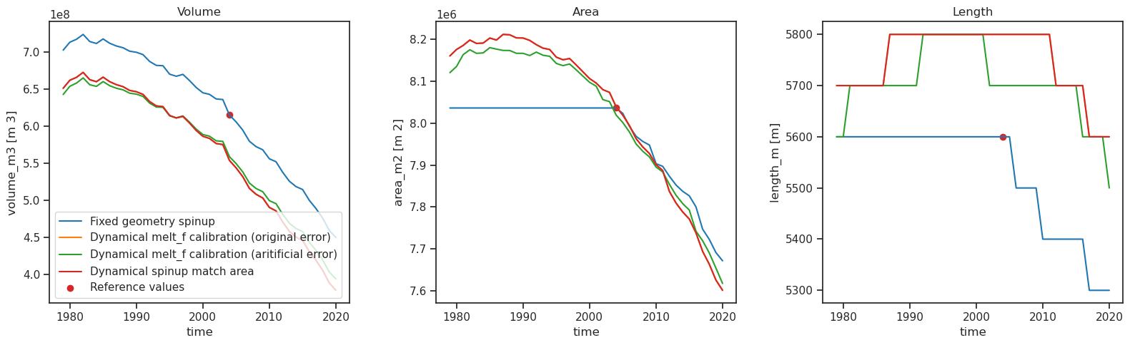
Also shown in the plots above is the dynamic melt_f calibration (including a dynamic spinup matching the area) in orange. However, you can not see an orange curve as it is exactly below the dynamic spinup matching the area (in green). The reason for this can be explained by comparing the reference geodetic mass balance (Hugonnet 2021) with the modelled ones, below the plots. You see that (by chance) the dynamic spinup already fits inside the provided observation uncertainty and therefore the dynamic melt_f calibration does not need to look further. But to showcase the ability of the dynamic melt_f calibration, we can artificially set the uncertainty lower and let it run again:
# define an artificial error for dmdtda
dmdtda_reference_error_artificial = 10 # error must be given as a positive number

tasks.run_dynamic_melt_f_calibration(gdir,
                                     ys=spinup_start_yr,  # When to start the spinup
                                     ye=2020,  # When the simulation should stop
                                     output_filesuffix='_dynamic_melt_f_artificial',  # Where to write the output
                                     ref_dmdtda=dmdtda_reference,  # user-provided geodetic mass balance observation
                                     err_ref_dmdtda=dmdtda_reference_error_artificial,  # uncertainty of user-provided geodetic mass balance observation
                                    );

with xr.open_dataset(gdir.get_filepath('model_diagnostics', filesuffix='_dynamic_melt_f_artificial')) as ds:
    ds_dynamic_melt_f_artificial = ds.load()
# plot again
y0 = gdir.rgi_date + 1

f, (ax1, ax2, ax3) = plt.subplots(1, 3, figsize=(16, 5))

ds_hist.volume_m3.plot(ax=ax1, label='Fixed geometry spinup');
ds_dynamic_melt_f.volume_m3.plot(ax=ax1, label='Dynamical melt_f calibration (original error)');
ds_dynamic_melt_f_artificial.volume_m3.plot(ax=ax1, label='Dynamical melt_f calibration (aritificial error)');
ds_dynamic_spinup_area.volume_m3.plot(ax=ax1, label='Dynamical spinup match area');
ax1.set_title('Volume');
ax1.scatter(y0, volume_reference, c='C3', label='Reference values');
ax1.legend();

ds_hist.area_m2.plot(ax=ax2);
ds_dynamic_melt_f.area_m2.plot(ax=ax2);
ds_dynamic_melt_f_artificial.area_m2.plot(ax=ax2);
ds_dynamic_spinup_area.area_m2.plot(ax=ax2);
ax2.set_title('Area');
ax2.scatter(y0, area_reference, c='C3')

ds_hist.length_m.plot(ax=ax3);
ds_dynamic_melt_f.length_m.plot(ax=ax3);
ds_dynamic_melt_f_artificial.length_m.plot(ax=ax3);
ds_dynamic_spinup_area.length_m.plot(ax=ax3);
ax3.set_title('Length');
ax3.scatter(y0, ds_hist.sel(time=y0).length_m, c='C3')

plt.tight_layout()
plt.show();

# and print out the modeled geodetic mass balances for comparision
def get_dmdtda(ds):
    yr0_ref_mb, yr1_ref_mb = ref_period.split('_')
    yr0_ref_mb = int(yr0_ref_mb.split('-')[0])
    yr1_ref_mb = int(yr1_ref_mb.split('-')[0])

    return ((ds.volume_m3.loc[yr1_ref_mb].values -
             ds.volume_m3.loc[yr0_ref_mb].values) /
            gdir.rgi_area_m2 /
            (yr1_ref_mb - yr0_ref_mb) *
            cfg.PARAMS['ice_density'])

print(f'Reference dmdtda 2000 to 2020 (original error):                      {dmdtda_reference:.2f} +/- {dmdtda_reference_error:6.2f} kg m-2 yr-1')
print(f'Reference dmdtda 2000 to 2020 (artificial error):                    {dmdtda_reference:.2f} +/- {dmdtda_reference_error_artificial:6.2f} kg m-2 yr-1')
print(f'Dynamical melt_f calibration dmdtda 2000 to 2020 (original error):   {get_dmdtda(ds_dynamic_melt_f):.2f}            kg m-2 yr-1')
print(f'Dynamical melt_f calibration dmdtda 2000 to 2020 (artificial error): {get_dmdtda(ds_dynamic_melt_f_artificial):.2f}            kg m-2 yr-1')
print(f'melt_f (original error):   {melt_f_original:.2f} kg m-2 day-1 °C-1')
print(f"melt_f (artificial error): {gdir.read_json('mb_calib')['melt_f']:.2f} kg m-2 day-1 °C-1")
Reference dmdtda 2000 to 2020 (original error):                      -1100.30 +/- 171.80 kg m-2 yr-1
Reference dmdtda 2000 to 2020 (artificial error):                    -1100.30 +/-  10.00 kg m-2 yr-1
Dynamical melt_f calibration dmdtda 2000 to 2020 (original error):   -1163.41            kg m-2 yr-1
Dynamical melt_f calibration dmdtda 2000 to 2020 (artificial error): -1090.44            kg m-2 yr-1
melt_f (original error):   5.00 kg m-2 day-1 °C-1
melt_f (artificial error): 4.89 kg m-2 day-1 °C-1
It is a made-up example, but you see that the dynamic melt_f calibration can match our ‘very accurate’ geodetic mass balance.
For additional options of the two run tasks have a look at their doc-strings (run_dynamic_spinup and run_dynamic_melt_f_star_calibration). You can also change all the settings of the included dynamic spinup inside the run_dynamic_melt_f_star_calibration by using kwargs_run_function (e.g. kwargs_run_function = {'minimize_for':'volume'} to match for volume instead of area).
Example where it is not working so well#
The dynamic spinup however is not always working that well, as the example below shows:
# now we switch to the 'bad' glacier
gdir = gdirs[1]
# We will "reconstruct" a possible glacier evolution from this year onwards
spinup_start_yr = 1979

# here we save the original melt_f_star for later
melt_f_star_original = gdir.read_json('mb_calib')['melt_f']

# and save some reference values we can compare to later
area_reference = gdir.rgi_area_m2  # RGI area
volume_reference = tasks.get_inversion_volume(gdir)  # volume after regional calibration to consensus
ref_period = cfg.PARAMS['geodetic_mb_period']  # get the reference period we want to use, 2000 to 2020
df_ref_dmdtda = utils.get_geodetic_mb_dataframe().loc[gdir.rgi_id]  # get the data from Hugonnet 2021
df_ref_dmdtda = df_ref_dmdtda.loc[df_ref_dmdtda['period'] == ref_period]  # only select the desired period
dmdtda_reference = df_ref_dmdtda['dmdtda'].values[0] * 1000  # get the reference dmdtda and convert into kg m-2 yr-1
dmdtda_reference_error = df_ref_dmdtda['err_dmdtda'].values[0] * 1000  # corresponding uncertainty
# ---- First do the fixed geometry spinup ----
tasks.run_from_climate_data(gdir,
                            fixed_geometry_spinup_yr=spinup_start_yr,  # Start the run at the RGI date but retro-actively correct the data with fixed geometry
                            output_filesuffix='_hist_fixed_geom',  # where to write the output
                            );
# Read the output
with xr.open_dataset(gdir.get_filepath('model_diagnostics', filesuffix='_hist_fixed_geom')) as ds:
    ds_hist = ds.load()

# ---- Second the dynamic spinup alone, matching area ----
tasks.run_dynamic_spinup(gdir,
                         precision_percent=3,  # For this glacier we only try to be within 3% or RGI_area
                         spinup_start_yr=spinup_start_yr,  # When to start the spinup
                         minimise_for='area',  # what target to match at the RGI date
                         output_filesuffix='_spinup_dynamic_area',  # Where to write the output
                         ye=2020,  # When the simulation should stop
                         );
# Read the output
with xr.open_dataset(gdir.get_filepath('model_diagnostics', filesuffix='_spinup_dynamic_area')) as ds:
    ds_dynamic_spinup_area = ds.load()

# ---- Third the dynamic spinup alone, matching volume ----
tasks.run_dynamic_spinup(gdir,
                         spinup_start_yr=spinup_start_yr,  # When to start the spinup
                         minimise_for='volume',  # what target to match at the RGI date
                         output_filesuffix='_spinup_dynamic_volume',  # Where to write the output
                         ye=2020,  # When the simulation should stop
                         );
# Read the output
with xr.open_dataset(gdir.get_filepath('model_diagnostics', filesuffix='_spinup_dynamic_volume')) as ds:
    ds_dynamic_spinup_volume = ds.load()
def plot_dynamic_spinup_bad_glacier():
    # Now make a plot for comparision
    y0 = gdir.rgi_date + 1

    f, (ax1, ax2, ax3) = plt.subplots(1, 3, figsize=(16, 5))

    ds_hist.volume_m3.plot(ax=ax1, label='Fixed geometry spinup');
    ds_dynamic_spinup_area.volume_m3.plot(ax=ax1, label='Dynamical spinup match area');
    ds_dynamic_spinup_volume.volume_m3.plot(ax=ax1, label='Dynamical spinup match volume');
    ax1.set_title('Volume');
    ax1.scatter(y0, volume_reference, c='C3', label='Reference values');
    ax1.legend();

    ds_hist.area_m2.plot(ax=ax2);
    ds_dynamic_spinup_area.area_m2.plot(ax=ax2);
    ds_dynamic_spinup_volume.area_m2.plot(ax=ax2);
    ax2.set_title('Area');
    ax2.scatter(y0, area_reference, c='C3')

    ds_hist.length_m.plot(ax=ax3);
    ds_dynamic_spinup_area.length_m.plot(ax=ax3);
    ds_dynamic_spinup_volume.length_m.plot(ax=ax3);
    ax3.set_title('Length');
    ax3.scatter(y0, ds_hist.sel(time=y0).length_m, c='C3')

    plt.tight_layout()
    plt.show();

    # and print out the modeled geodetic mass balances for comparision
    def get_dmdtda(ds):
        yr0_ref_mb, yr1_ref_mb = ref_period.split('_')
        yr0_ref_mb = int(yr0_ref_mb.split('-')[0])
        yr1_ref_mb = int(yr1_ref_mb.split('-')[0])

        return ((ds.volume_m3.loc[yr1_ref_mb].values -
                 ds.volume_m3.loc[yr0_ref_mb].values) /
                gdir.rgi_area_m2 /
                (yr1_ref_mb - yr0_ref_mb) *
                cfg.PARAMS['ice_density'])

plot_dynamic_spinup_bad_glacier()
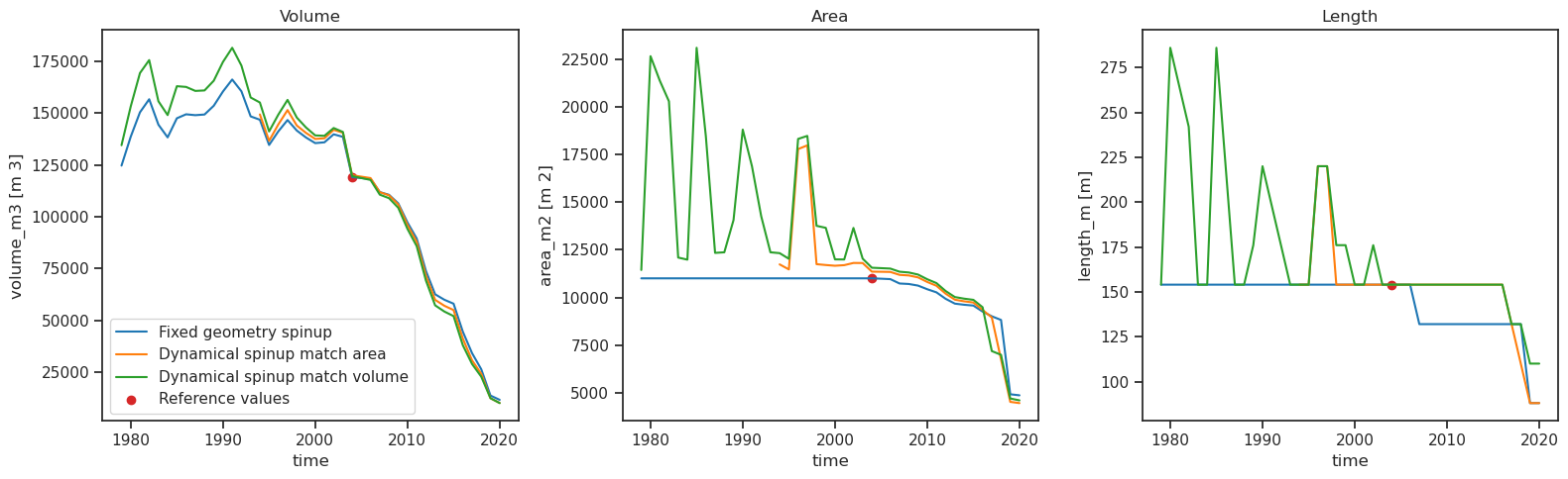
In this example, you see that the dynamic spinup run matching area does not start in 1980. The reason for this are the two main problems and the coping strategy of reducing the spinup time, described here in more detail.
To get an glacier evolution starting at 1980 you can use add_fixed_geometry_spinup = True:
tasks.run_dynamic_spinup(gdir,
                         precision_percent=3,  # For this glacier we only try to be within 3% or RGI_area
                         spinup_start_yr=spinup_start_yr,  # When to start the spinup
                         minimise_for='area',  # what target to match at the RGI date
                         output_filesuffix='_spinup_dynamic_area',  # Where to write the output
                         ye=2020,  # When the simulation should stop
                         add_fixed_geometry_spinup=True,  # add a fixed geometry spinup if period needs to be shortent
                         );

with xr.open_dataset(gdir.get_filepath('model_diagnostics', filesuffix='_spinup_dynamic_area')) as ds:
    ds_dynamic_spinup_area = ds.load()

plot_dynamic_spinup_bad_glacier()
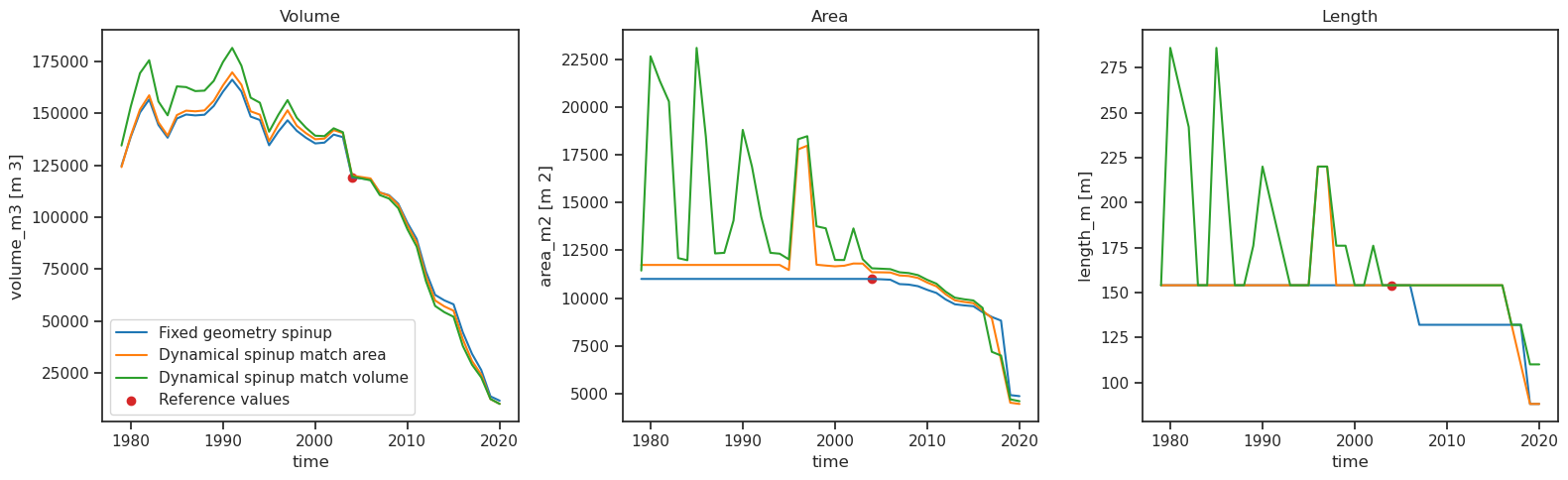
You see that a fixed geomtery was added to the dynamical spinup matching the area (orange curve). With this you can be sure that all glaciers start at the same year.
Dynamical spinup and hydrological output#
Fortunately, it is also possible to run the spinup model with additional hydrological output:
# Here we use Hintereisferner again
gdir = gdirs[0]

cfg.PARAMS['store_model_geometry'] = True  # This is required for the hydro runs

# Dynamic melt_f calibration including a dynamic spinup to match for area
tasks.run_with_hydro(gdir,
                     run_task=tasks.run_dynamic_melt_f_calibration,  # The task to run with hydro
                     ys=spinup_start_yr,  # When to start the spinup
                     ye=2020,  # When the simulation should stop
                     store_monthly_hydro=True,  # compute monthly hydro diagnostics
                     ref_area_from_y0=True,  # Even if the glacier may grow, keep the reference area as the year 0 of the simulation
                     output_filesuffix='_spinup_dynamic_hydro',  # Where to write the output - this is needed to stitch the runs together afterwards
                     );

# Read the output
with xr.open_dataset(gdir.get_filepath('model_diagnostics', filesuffix='_spinup_dynamic_hydro')) as ds:
    ds_dynamic_spinup_hydro = ds.load()

ds_dynamic_spinup_hydro = ds_dynamic_spinup_hydro.isel(time=slice(0, -1))  # The last timestep is incomplete for hydro (not started)
2023-08-27 23:33:04: oggm.cfg: PARAMS['store_model_geometry'] changed from `False` to `True`.
Annual runoff#
The new hydrological variables are now available. Let’s make a pandas DataFrame of all “1D” (annual) variables:
sel_vars = [v for v in ds_dynamic_spinup_hydro.variables if 'month_2d' not in ds_dynamic_spinup_hydro[v].dims]
df_annual = ds_dynamic_spinup_hydro[sel_vars].to_dataframe()
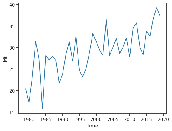
The hydrological variables are computed on the largest possible area that was covered by glacier ice in the simulation. This is equivalent to the runoff that would be measured at a fixed-gauge station at the glacier terminus. The total annual runoff is:
# Select only the runoff variables and convert them to megatonnes (instead of kg)
runoff_vars = ['melt_off_glacier', 'melt_on_glacier', 'liq_prcp_off_glacier', 'liq_prcp_on_glacier']
df_runoff = df_annual[runoff_vars] * 1e-9
df_runoff.sum(axis=1).plot(); plt.ylabel('Mt');
It consists of the following components:
melt off-glacier: snow melt on areas that are now glacier free (i.e. 0 in the year of largest glacier extent, in this example at the start of the simulation)
melt on-glacier: ice + seasonal snow melt on the glacier
liquid precipitaton on- and off-glacier (the latter being zero at the year of largest glacial extent, in this example at start of the simulation)
f, ax = plt.subplots(figsize=(10, 6));
df_runoff.plot.area(ax=ax, color=sns.color_palette("rocket")); plt.xlabel('Years'); plt.ylabel('Runoff (Mt)'); plt.title(rgi_ids[0]);
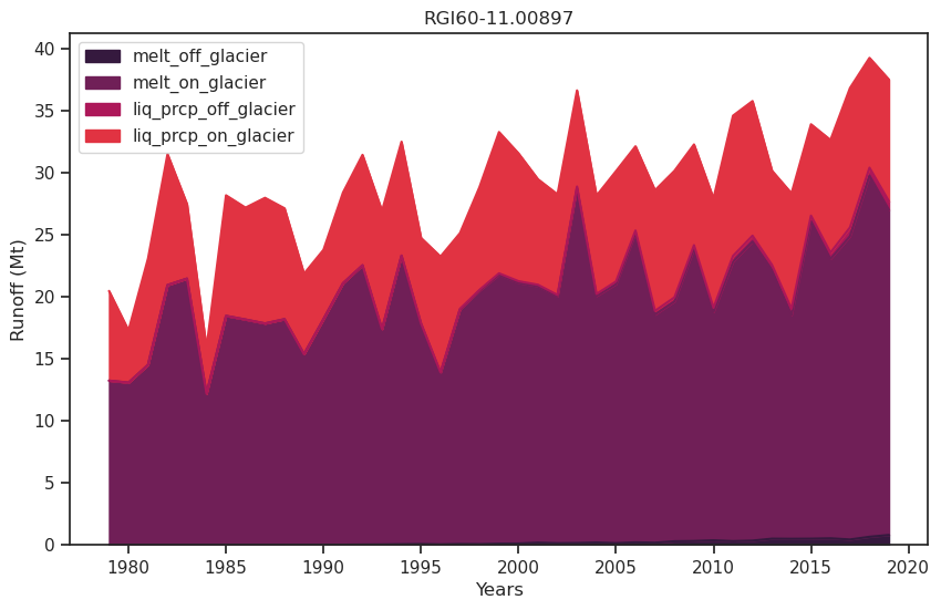
As the glacier retreats, total runoff decreases as a result of the decreasing glacier contribution.
Monthly runoff#
The “2D” variables contain the same data but at monthly resolution, with the dimension (time, month). For example, runoff can be computed the same way:
# Select only the runoff variables and convert them to megatonnes (instead of kg)
monthly_runoff = ds['melt_off_glacier_monthly'] + ds['melt_on_glacier_monthly'] + ds['liq_prcp_off_glacier_monthly'] + ds['liq_prcp_on_glacier_monthly']
monthly_runoff *= 1e-9
monthly_runoff.clip(0).plot(cmap='Blues', cbar_kwargs={'label':'Mt'}); plt.xlabel('Months'); plt.ylabel('Years'); plt.title(rgi_ids[0]);
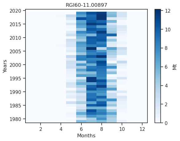
See hydrological_output for more info on how to interpret the hydrological output!
What’s next?#
return to the OGGM documentation
back to the table of contents